Ray Optics Module Updates
For users of the Ray Optics Module, COMSOL Multiphysics® version 5.3 brings a new Ray Termination feature to eliminate unnecessary rays, functionality to import photometric data, and a new simulation app for designing a solar dish receiver. See all of the Ray Optics Module updates in more detail below.
Ray Termination Feature
The new Ray Termination feature can be used to annihilate rays without requiring them to stop at a boundary. The rays can be terminated as they exit a bounding box, which can be based on the geometry or user-defined spatial extents. You can use the Ray Termination feature to discard unnecessary information about the ray paths and remove clutter from the trajectory plots. Beyond geometrical constraints, rays can be terminated if their intensity or power becomes smaller than a specified threshold, or if they stray too far from the model geometry. This feature can be employed to avoid using excessive computational resources on rays that have become attenuated due to the presence of absorbing media and rays that have extremely low intensity due to interaction with curved surfaces.
A collimated beam is focused by an uncoated convex lens. The Ray Termination feature is used to terminate the stray light that is reflected by the lens surfaces. The color expression is proportional to the log of the ray intensity.
*Rays propagating through two convex lenses with focal lengths of 200 mm (top) and 100 mm (bottom). The rays passing through the lens with a shorter focal length decrease in intensity more rapidly past the focal point, so they are terminated by the _Ray Termination_ feature, while the rays passing through the lens with a longer focal length continue to propagate.
Import Photometric Data Files
It is possible to specify nonuniform distributions of ray intensity and power by importing photometric data files into a ray optics model. The Photometric Data File feature supports the .ies file extension, the standard photometric data file format of the Illuminating Engineering Society of North America (IESNA). To use this feature, select Photometric Data Import for the Intensity initialization in the Total Source Power section of the Release from Grid node.
When the photometric data file is imported into a model, it generates a set of functions that are used to initialize the ray intensity and power as a function of the initial ray direction. You can specify directions for the photometric horizontal and photometric zero, which indicate the orientation of the lamp according to IES standards.
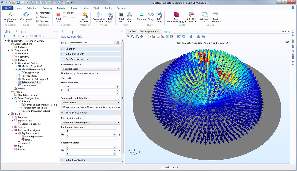
Rays are released in a hemispherical distribution about the z-axis. The color expression is proportional to the ray intensity, which is generated from the imported photometric data file.
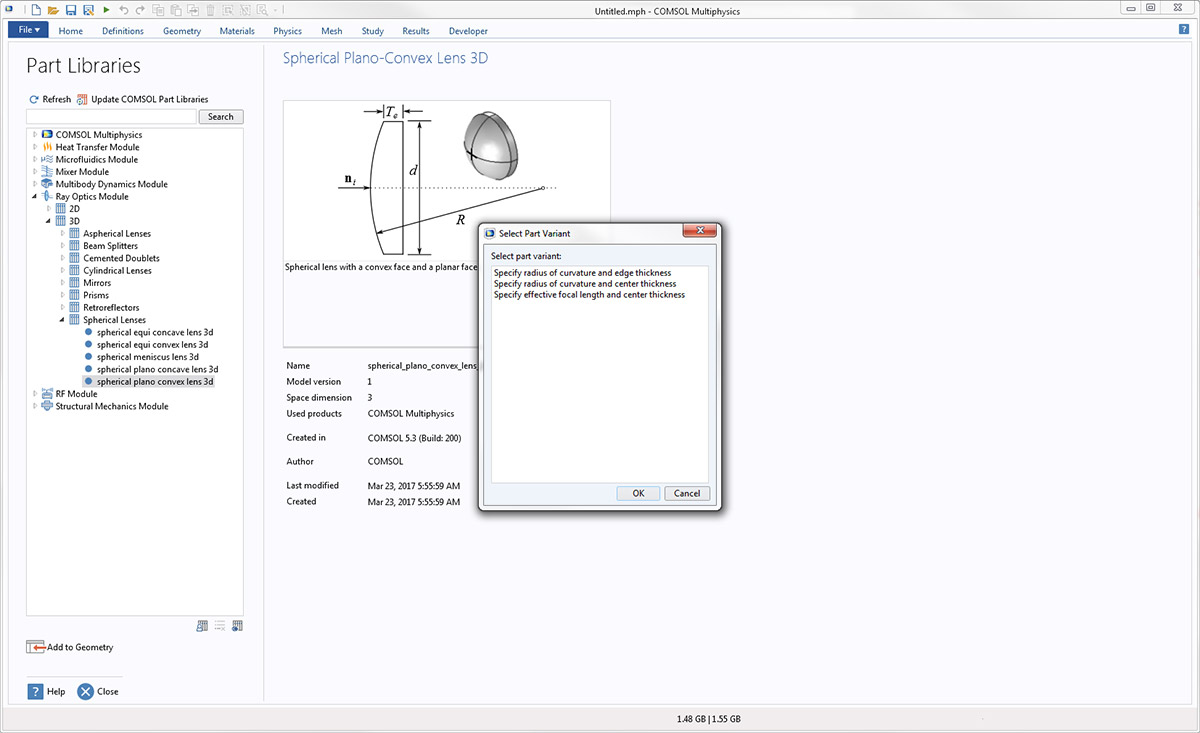
Geometry Part Variants
There are now several different ways to specify the dimensions of geometry parts in the dedicated Part Library for the Ray Optics Module. You can select which combination of input parameters, or part variants, you would like to use when you load the part into the model. When you click Add to Geometry, a dialog box will appear that prompts you to select the part variant.
New Geometry Parts: Compound Parabolic Concentrators
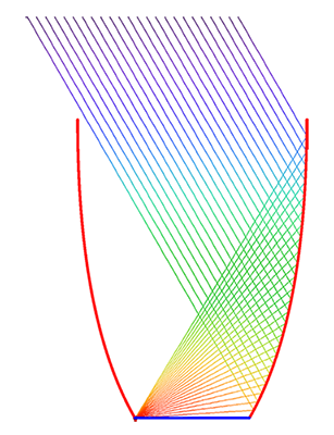
The Part Library for the Ray Optics Module now includes the Compound Parabolic Concentrator (CPC). The CPC has parabolic surfaces that are positioned close enough together so that the end of each side is located at the focal point of the opposite side. Light that is incident at anything less than a specified angle, called the acceptance half-angle, will always be transmitted through the concentrator, making it a useful tool for focusing incoming radiation from several different directions.
 When rays are incident at an angle equal to the acceptance half-angle of the CPC, they converge toward the focus on the opposite side.
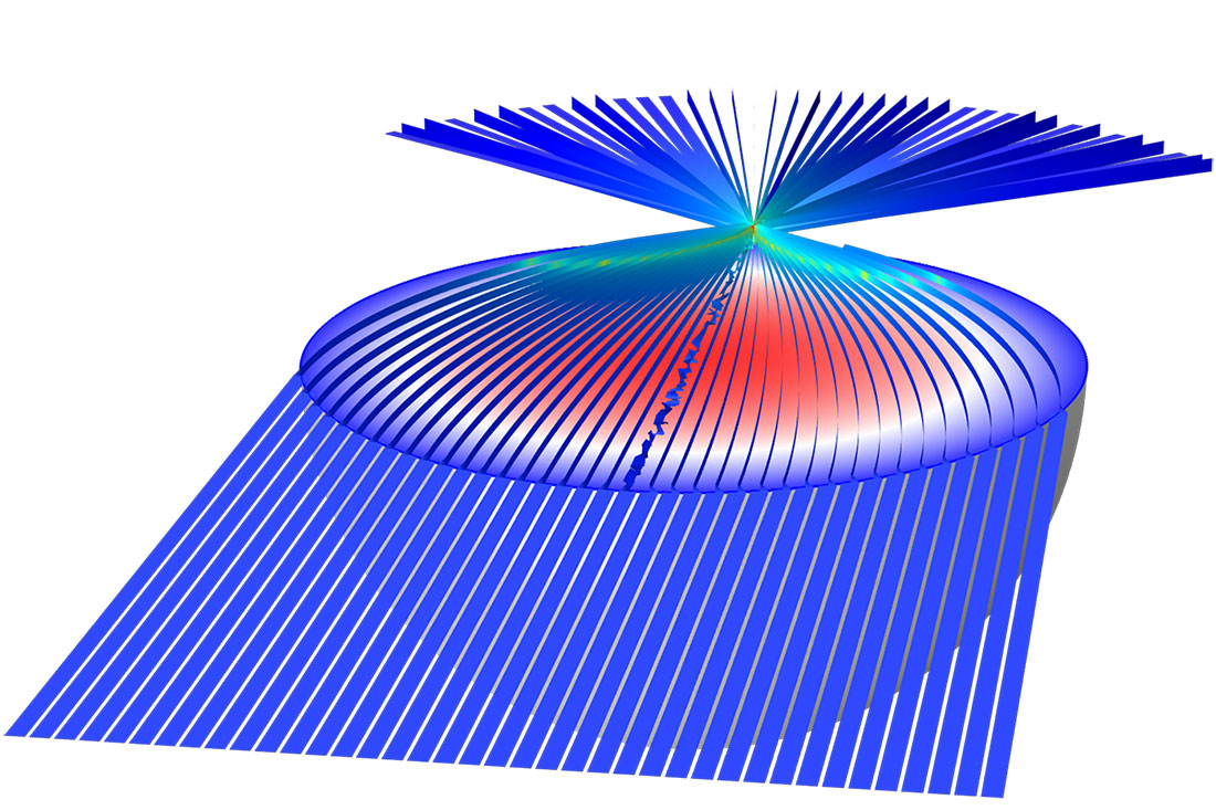
Rays are released into the CPC following a conical distribution. Because the cone angle is less than the acceptance half-angle, all rays are focused by the parabolic surfaces and reach the output (shown as a blue line)
Lambertian Emission
The ray release features now include an option to release rays with a Lambertian distribution of initial directions. Rays are released with initial directions based on Lambert's cosine law.
Lambert's cosine law states that the probability that a ray will be released through a differential solid angle element dω with polar angle θ is proportional to cos θ. By comparison, in the isotropic hemispherical distribution, the ray is equally likely to be released through any differential solid angle in the hemisphere.
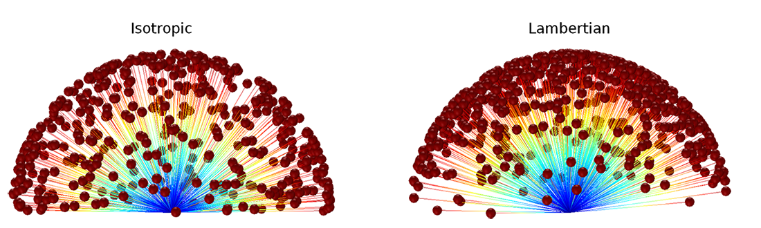 Comparison of ray distributions in an isotropic hemispherical release (left) and a Lambertian release (right).
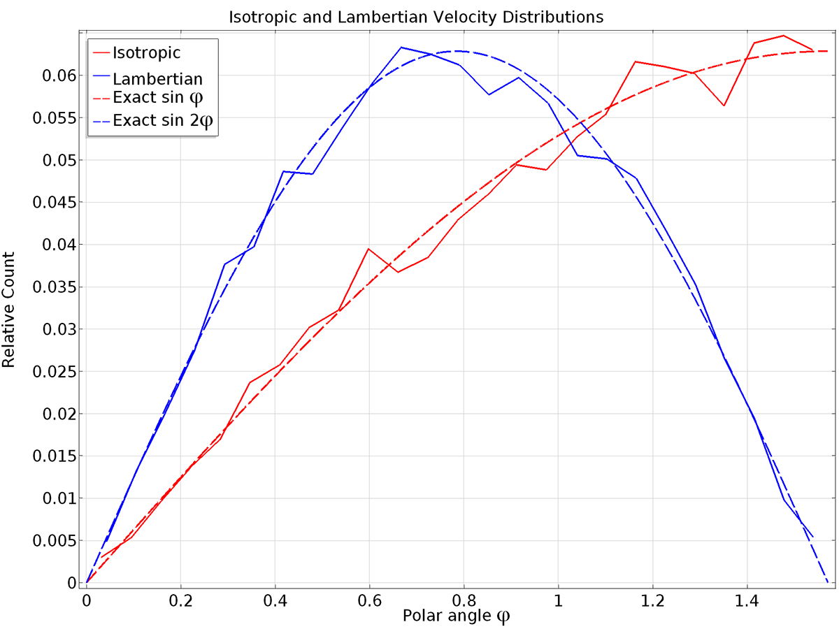 Histogram of the polar angles in the isotropic and Lambertian distributions.
Improved Ray Tracing in 2D Axisymmetric Geometries
When computing ray intensity in 2D axisymmetric models, the wavefront associated with the propagating ray is now treated as a spherical or ellipsoidal wave instead of a cylindrical wave (which is only an appropriate simplification in true 2D models). In other words, the principal radius of curvature associated with the azimuthal direction is computed for all rays. This leads to more realistic calculations of ray intensity in 2D axisymmetric models.
In addition, dedicated release features are now available to release rays from edges, points, or at specified coordinates along the axis of symmetry. When using one of these dedicated release features, a built-in option is available to release rays in an anisotropic hemisphere such that each ray subtends approximately the same solid angle in 3D.
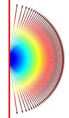 When using the option to release a spherical distribution of rays from the axis of symmetry, rays are weighted more heavily in the radial direction so that the solid angle subtended by each ray in 3D is roughly equal. The axis of symmetry is shown as a solid red line.
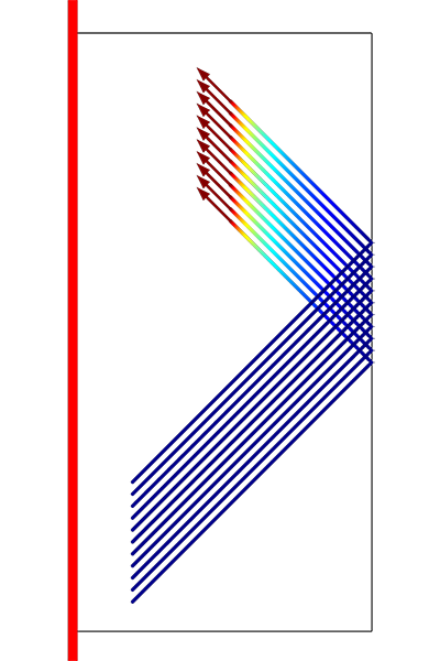 Specular reflection for a plane wave in a 2D axisymmetric model. The axis of symmetry is shown as a solid red line. The color expression shows the ray intensity. Even though the boundary is a straight edge, the rays increase in intensity after being reflected because the boundary is treated as a surface of revolution for the purpose of computing wavefront curvatures.
Ribbons on Ray Trajectories
It is now possible to render ray paths as ribbons in the Ray Trajectories plot. You can specify the orientation and thickness of the ribbon. For example, when rays propagate through graded-index media, the ribbons can be oriented normal to or parallel with the plane containing the curved ray paths.
 Ray propagation through a Luneburg lens, a graded-index medium. Rays that do not pass through the symmetry axis of the lens follow curved paths. Here, the ribbon orientation is normal to the plane containing the ray paths and the color is proportional to the ray intensity.
Extra Time Steps in Trajectory Plots
When plotting ray trajectories, it is now easier than ever to plot additional time steps that correspond to ray-wall interaction times. The number of these extra time steps can now be controlled directly from the Settings window for the Ray Trajectories plot. Built-in options are available to specify the maximum number of extra time steps directly or as a multiple of the number of stored solution times.
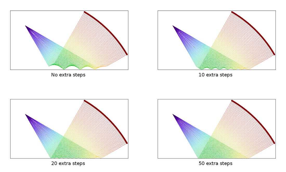 As the number of extra time steps in the trajectory plot is increased, the times at which each ray bounces off the wall can be seen more clearly.
Ray Detector Feature
The Ray Detector feature is a domain or boundary feature that provides information about rays arriving on a set of selected domains or surfaces from a release feature. Such quantities include the number of rays transmitted and the transmission probability, or the ratio of the number of transmitted rays to the number of released rays. It is possible to count all rays or only those rays released by a specific physics feature. The feature provides convenient expressions that can be used in the Filter attribute of the Ray Trajectories plot, which allows only the rays that reach a specified set of domains or boundaries to be visualized.
The following variables are defined by an instance of the Ray Detector feature with the feature tag <tag>:
- <tag>Nsel_: number of transmitted rays from the release feature to the detector
- <tag>.alpha_: the transmission probability from the release feature to the detector
- <tag>.rL_: a logical expression for ray inclusion; this can be set in the Filter attribute of the Ray Trajectories plot in order to visualize the rays that connect the radiation source to the detector
Rays are released isotropically from a point source and are reflected specularly until they hit an absorbing surface (marked in red). Using a Ray Detector it is easy to define filter expressions to show only those rays that hit the absorbing surface (bottom).
Extra Selections in Physics Features
For some physics features, such as the Grating, Linear Polarizer, Linear Wave Retarder, and Mueller Matrix features, it is sometimes necessary to specify an edge selection in addition to the boundary selection of the physics feature. Typically, this edge selection is used to indicate the orientation of a diffraction grating or optical component in 3D. In previous versions of COMSOL Multiphysics®, the edge selection was specified by adding a Reference Edge subnode to the physics feature. In version 5.3, however, the edge selection has been moved to a dedicated section in the Settings window for the parent physics feature. This provides a more transparent layout of the user interface in which selections of different geometric entity levels can be viewed in the same window.
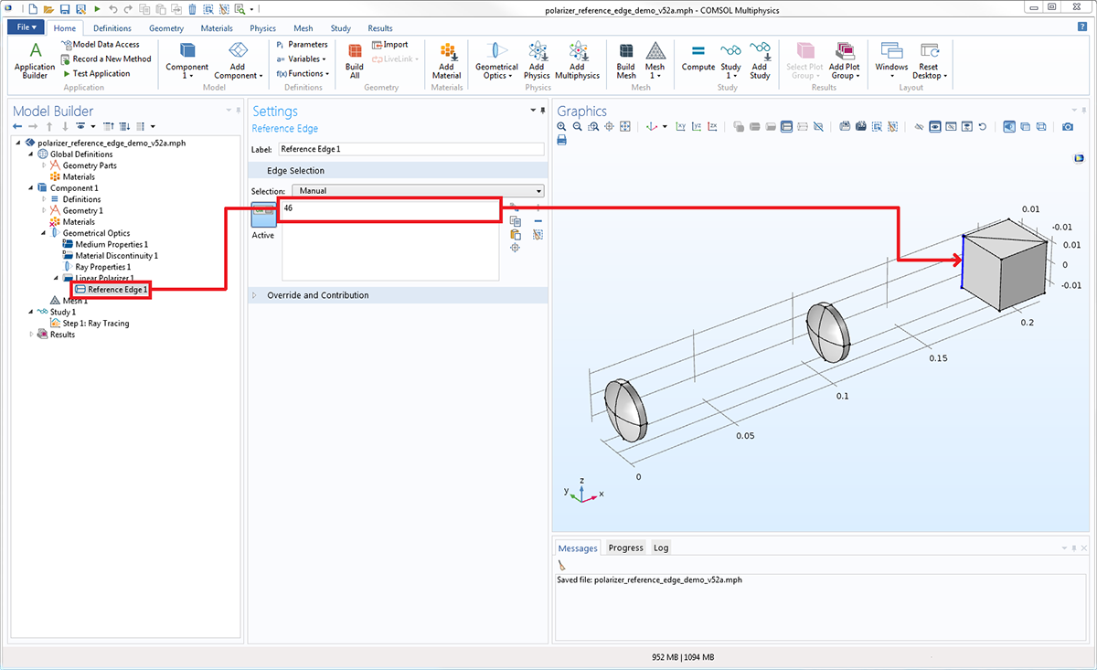
In COMSOL Multiphysics® version 5.2a, the orientation of a linear polarizer was specified by adding the Reference Edge subnode.
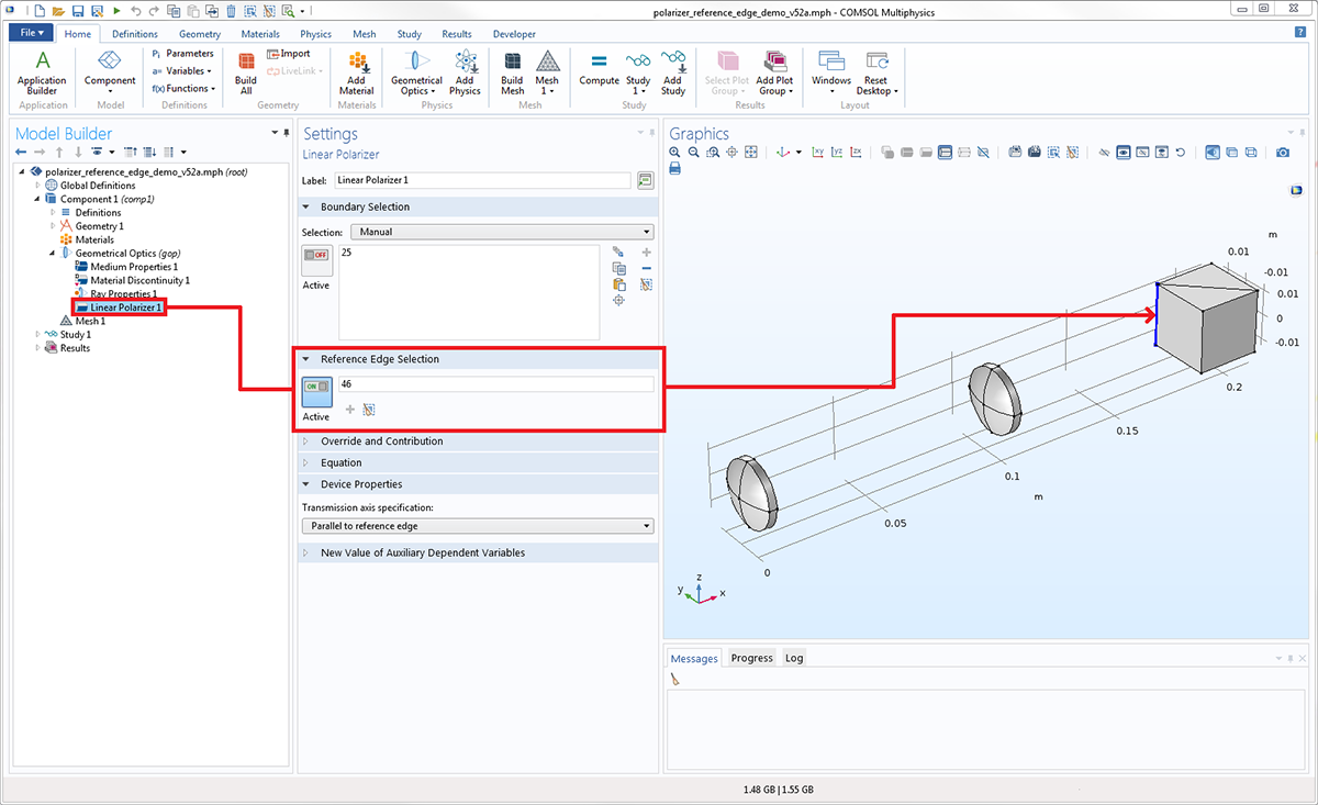
In COMSOL Multiphysics® version 5.3, the orientation of the linear polarizer is determined by a second selection in the Settings window for the Linear Polarizer node.
Improvements to the Optical Aberration Plot
When plotting linear combinations of monochromatic aberrations on the unit circle with the Optical Aberration plot, you can specify the position of the unit circle. By entering different positions for several unit circles, you can view multiple types of aberrations in the Graphics window at the same time. Further, the Optical Aberration plot now supports the Height Expression plot attribute. Use this to render the 2D aberration plot in a 3D canvas with height proportional to the combination of Zernike polynomials.
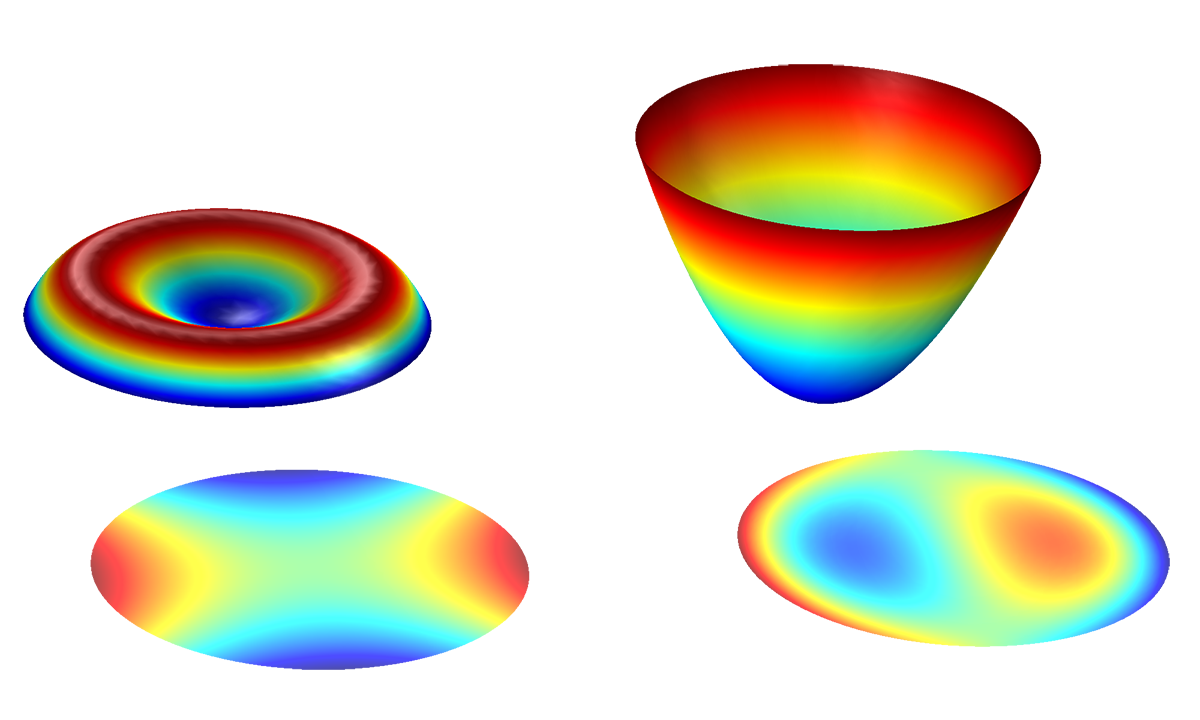 Plot of four aberrations, using height expressions and different unit circle positions. The terms shown are the spherical aberration (top-left), defocus (top-right), astigmatism (bottom-left), and vertical coma (bottom-right).
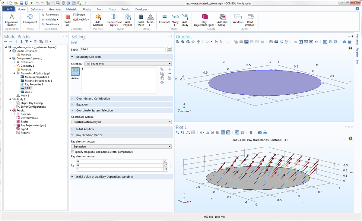
Coordinate System Selection for Inlets
When releasing rays at a boundary using the Inlet feature, you can initialize the particle velocity or momentum using any coordinate system that has been defined for the model component.
New Component Couplings on Rays
New component couplings are automatically created for each instance of the Geometrical Optics interface, and the behavior of the old component couplings has changed. The old component couplings, for example gop.gopop1(expr), now automatically exclude rays that have not yet been released and rays that have disappeared. The degrees of freedom of such rays are usually not-a-number (NaN), so it is convenient to automatically exclude them when evaluating sums and averages over the rays.
| Name | Description |
|---|---|
|
Sum of expression |
|
Sum of expression |
|
Average of expression |
|
Average of expression |
|
Maximum of expression |
|
Maximum of expression |
|
Minimum of expression |
|
Minimum of expression |
|
Evaluate |
|
Evaluate |
|
Evaluate |
|
Evaluate |
Additional Statistics Based on Ray Status
When the Store ray status data check box is selected, the following new variables will be defined.
Note: The expressions are written for an instance of the Geometrical Optics interface with tag gop. Physics interface tags will naturally be different for different physics interfaces.
| Name | Expression | Description |
|---|---|---|
|
|
Fraction of rays frozen at final time |
|
|
Fraction of rays stuck at final time |
|
|
Fraction of rays active at final time |
|
|
Fraction of rays disappeared at final time |
|
|
Fraction of secondary rays released at final time |
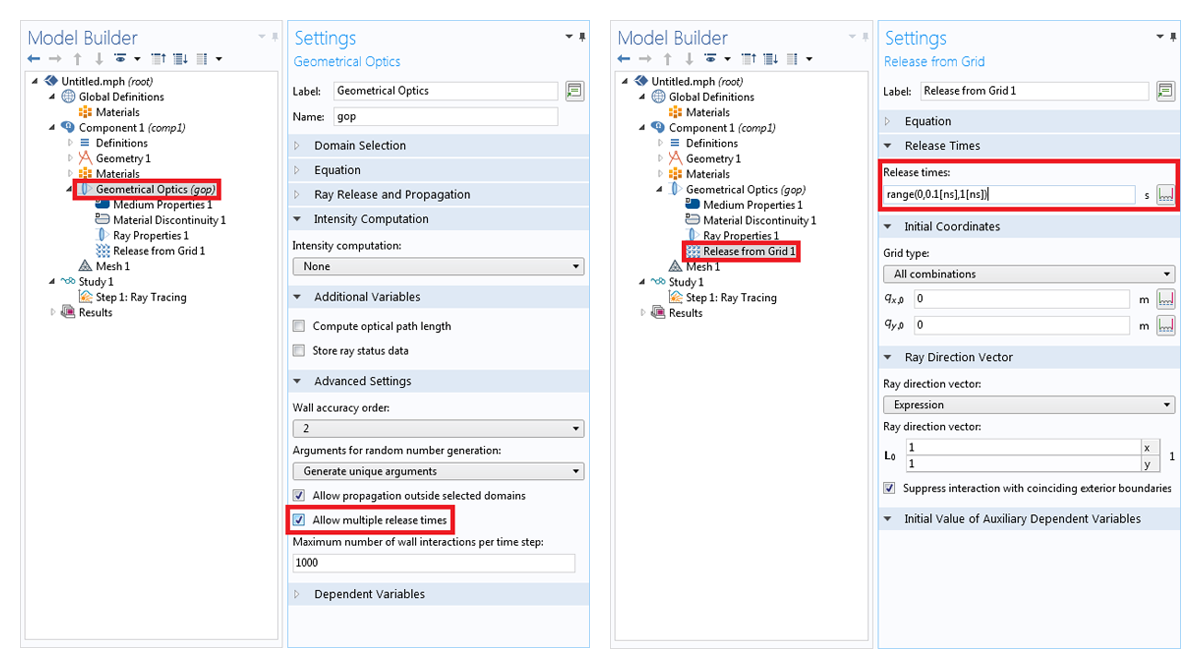
Advanced Options to Specify Ray Release Times
You can now enter a range of different ray release times. In previous versions, all rays had to be released at the same time. To enable specification of different release times, select the Allow multiple release times check box in the Advanced Settings section of the Geometrical Optics interface Settings window. Then, in the release feature node, you can specify a range of release times.
Convergence-Based Termination Criteria for Bidirectionally Coupled Models
For models that use the Bidirectionally Coupled Particle Tracing study step to iterate between stationary and ray tracing solutions, you can now terminate the solver loop based on a convergence criterion instead of a fixed number of iterations.
New App: Solar Cavity Receiver Designer
Solar concentrator/cavity receiver systems can be used to focus incident solar radiation into a small region, generating intense heat. This heat can then be converted to electrical or chemical energy. A common figure-of-merit in solar thermal power systems is the concentration ratio, or the ratio of the solar flux on the surface of the receiver or in the focal plane to the ambient solar flux.
The Solar Cavity Receiver Designer is a runnable application based on the Solar Dish Receiver tutorial model. In this app, incident solar radiation is reflected by a parabolic dish, while the concentrated solar radiation is collected in a small cavity. A total of six different parameterized cavity geometries are available for investigation: Cylindrical, Dome, Heteroconical, Elliptical, Spherical, and Conical. It is also possible to take several different types of perturbation into account, including solar limb darkening and surface roughness. For each cavity geometry, built-in plots show the flux distribution and concentration ratio in the focal plane as well as the incident flux on the interior surfaces of the cavity.
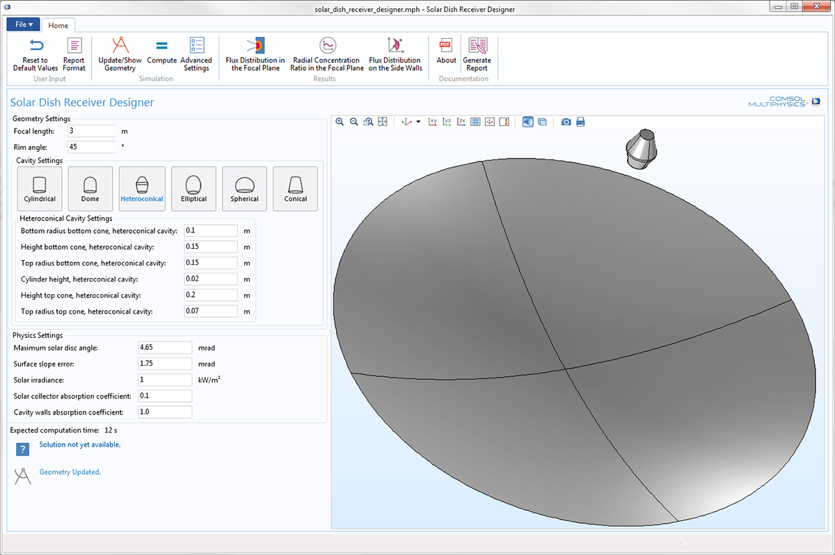 The Solar Cavity Receiver Designer app. The geometry shown consists of a parabolic reflector facing the sun and a heteroconical cavity receiver.
Application Library path for the Solar Cavity Receiver Designer app:
Ray_Optics_Module/Applications/solar_dish_receiver_designer
New Tutorial Model: Total Internal Reflection Thin-Film Achromatic Phase Shifter (TIRTF APS)
The capability to alter the polarization of light is crucial to a wide variety of optical devices. For example, the polarization of light has a significant effect on the performance of optical isolators, attenuators, and beam splitters. By assigning a specific polarization to light, most notably linear or circular polarization, it is possible to substantially reduce glare in optical systems.
One of the most fundamental methods of manipulating polarization is wave retardation in which one component of the electric field is subjected to a phase delay, or retarded, relative to the orthogonal electric field component in a propagating beam of light. In this tutorial, the phenomenon of total internal reflection is used to design and model an achromatic phase shifter, or a wave retarder that exhibits nearly uniform phase delay over a wide spectral range. The phase retardation is affected by the presence of thin dielectric layers on the boundary between the two media.
In this benchmark model, phase retardation angles for single- and triple-layer coatings are computed and compared against published results. This principle can be used to design a total internal reflection thin-film achromatic phase shifter (TIRTF APS) with nearly uniform phase retardation over a wide spectral range.
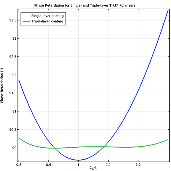 Phase retardation is plotted as a function of free-space wavelength. The phase retardation can be made more uniform over a wide spectral range if a multilayer dielectric coating is applied to the reflecting surface.
Application Library path for the Achromatic Phase Shifter tutorial model:
Ray_Optics_Module/Polychromatic_Light/achromatic_phase_shifter
New Tutorial Model: Fresnel Rhomb
A Fresnel rhomb is a prism that utilizes total internal reflection to manipulate the polarization of light. In this example, light in the prism is internally reflected at an angle of incidence that induces a 45-degree phase delay between s- and p-polarized radiation. By subjecting the light to two such reflections, the prism converts incoming linearly polarized light to circularly polarized light.
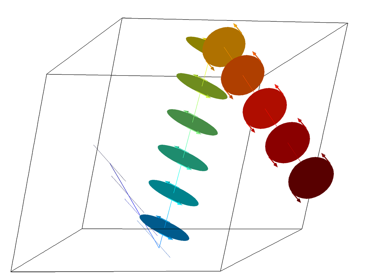 Polarization ellipses of a ray in the Fresnel rhomb. The ray is initially linearly polarized, with its polarization at a 45-degree angle to the plane of incidence, and then becomes elliptically polarized after one reflection and circularly polarized after two reflections.
Application Library path for the Fresnel Rhomb tutorial model:
Ray_Optics_Module/Tutorials/fresnel_rhomb