Postprocessing and Visualization Updates
COMSOL Multiphysics® version 5.3 brings rendering and visualization improvements that will make postprocessing your results easier and more effective. The Selection tool is now available for individual plots as well as for entire data sets, 1D plots can have two y-axes for results with different scales, and results with multiple parameters are easier to view with the Plot Next and Plot Previous buttons. Check out all of the rendering and visualization updates included in COMSOL Multiphysics® version 5.3 below.
Using Selections as a Plot Attribute
The Selection feature makes it easier to filter a plot to a subset of a model's geometry. Previously only available as an attribute for the Data Set node, you can now add the Selection feature for specific plots, rather than just for the data set itself. This means that you can be more discriminating in what geometric components you choose to make a part of your results visualizations. In the image from the Car Windshield Antenna Effect on a Cable Harness example from the RF Module, the Selection feature has been used to specify the electric field norm as a surface plot on the harness of a car affected by electromagnetic radiation. The removed surfaces that allow the harness to be visible can also be hidden using the Selection feature for plots.
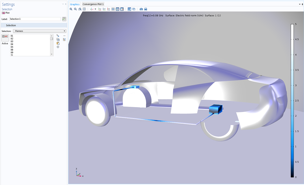
Radiation emitted from an antenna induces an electric current on the outer surface of the cable harness in a car. A group of surfaces that make up the harness have been gathered under the Harness Selection, and a surface plot of this selection can be chosen in order to illustrate the electric field norm on this component (Jupiter Aurora Borealis color table).
Application Library paths for examples using the Plot selection attribute:
RF_Module/Antennas/car_emiemc
RF_Module/Antennas/patch_antenna
Plot Different Quantities on Two Y-Axes
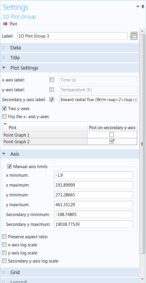
Presenting multiple and comparative results and data from your simulations has become easier to do through just a couple of clicks. You can now plot quantities of different scales on both y-axes of 1D plots against a parameter value on the x-axis. To make use of this functionality, select the Two y-axes check box in the Settings window of a 1D Plot Group node and then select the variable that you would like to add to the second y-axis (see image).
A new feature has also been introduced for when you are plotting 1D plot groups: the ability to switch the quantity on the y-axis to instead be presented on the x-axis and vice versa. In this case, you would select the Flip the x- and y-axes check box in the Settings window of a 1D Plot Group node (see image).
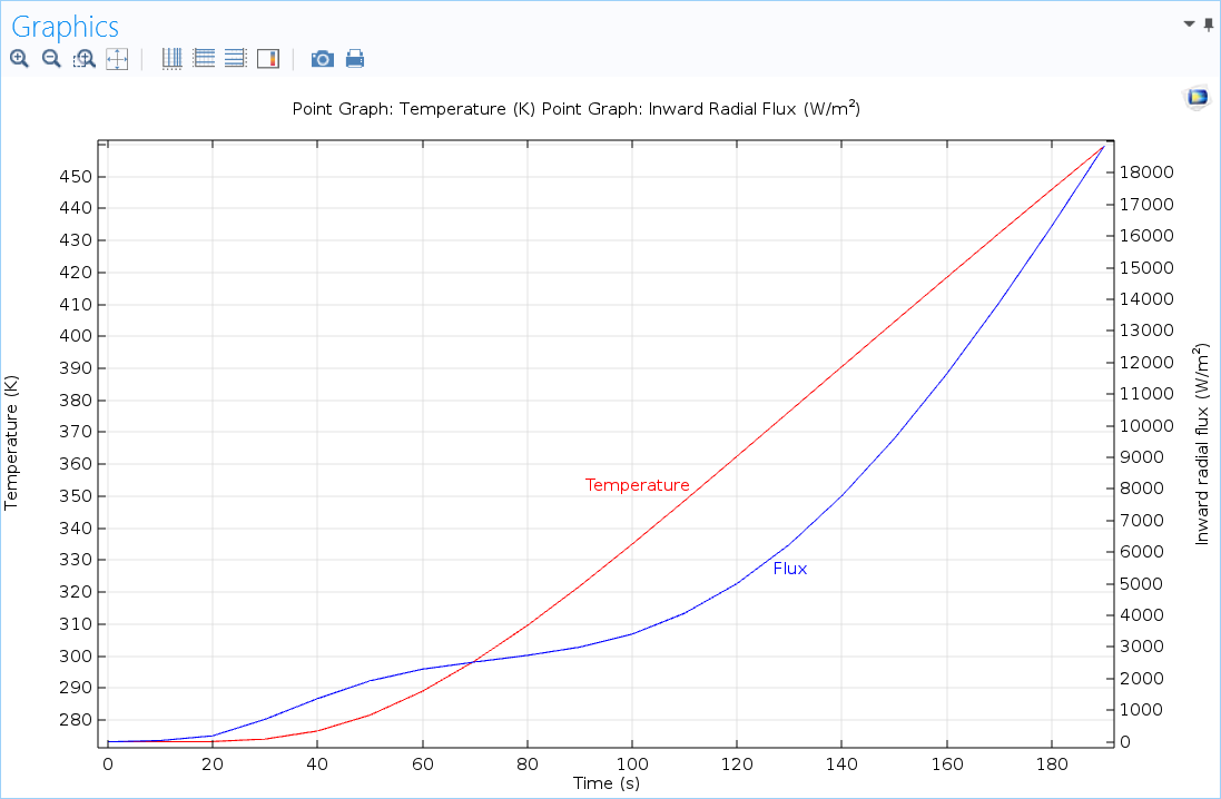
Plots of the temperature (left y-axis) and heat flux (right y-axis) from a time-dependent heat transfer simulation.
Application Library paths for examples using the Two y-axes feature:
Batteries_and_Fuel_Cells_Module/Thermal_Management/li_battery_thermal_2d_axi
Plasma_Module/Global_Discharges/chlorine_global_model
Step Between Solutions Using Toolbar Buttons
Viewing a list of times for a time-dependent solution or a parameter list from a parametric solution has become more flexible with the Plot Previous and Plot Next toolbar buttons. Previously, when multiple plots were able to be visualized over a range of values, you had to select the different parameter values from drop-down menus to see the sequence of changing plots or else view them all as an animation. The new Plot Previous and Plot Next toolbar buttons allow you to easily and quickly step between solutions in models presenting time-dependent, parametric sweep, or eigenvalue analyses, to name a few. The keyboard shortcuts F6 and F7 can be very useful as an ergonomic alternative to clicking.
Streamline Surface Plot
Sometimes, streamline plots do not give an adequate picture of the intricacies involved in a 3D field — in particular, one displaying fluid flow. With streamlines going in all directions at once, it can be hard to investigate a flow field at a surface, in an area where flow is dominating or is almost stagnant, or where flow is affected by a part within the modeling domain. The new Streamline surface plot type shows streamlines on a planar surface in a 3D model. This gives you more control over where to visualize your flow results and provides better understanding of the flow field. You can easily select an existing planar surface to plot your streamlines on or define a cut plane where they will be visualized.
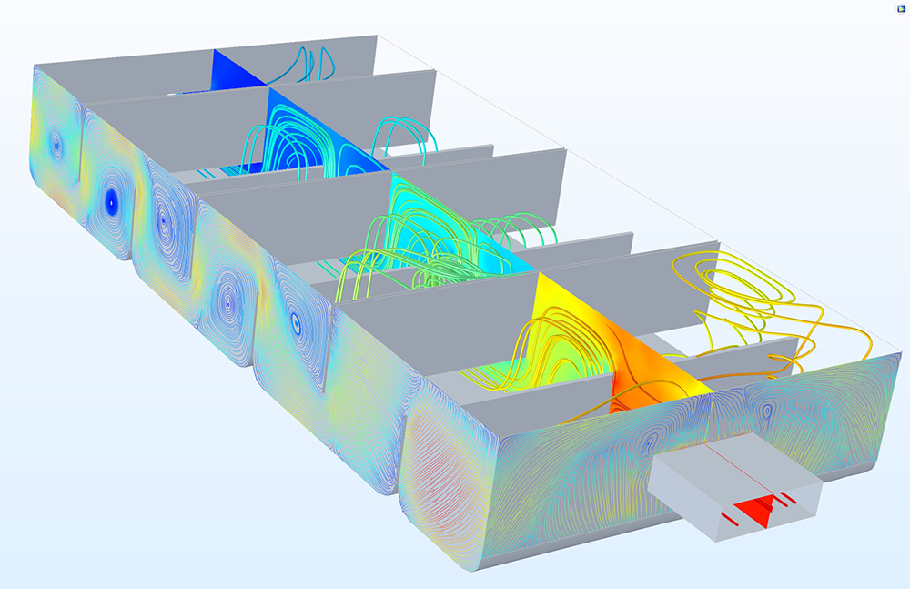
This model of a water treatment basin uses a Streamline surface plot type on a surface close to the wall of the reactor to show the flow field in this potentially stagnant region. It has been combined with a 3D streamline plot showing a representation of the flow field throughout the reactor as well as a planar plot of the pressure field. All three plot types use the Rainbow color table to show magnitudes.
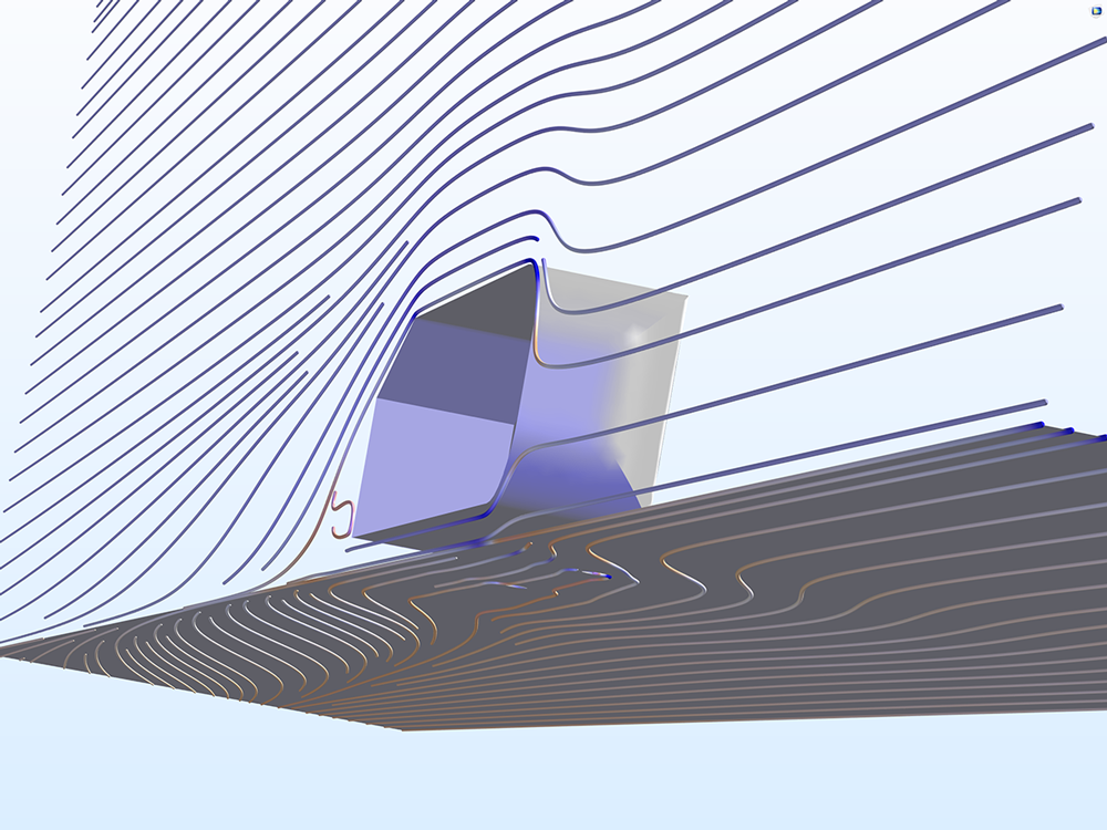
The model domain of the example of flow past a representation of a vehicle includes a symmetry plane and a bottom boundary (the road, if you like). This image shows the Streamline surface plot using the Twilight color table for the flow on the symmetry plane and a plane just above the surface of the road.

A Streamline surface plot using the Jupiter Aurora Borealis color table in a plane of a mixer app. At this instance in time, the streamline plot shows the flow field as it is affected by the blades of the mixer.
Beam Width Calculation
You can now compute the beam width and the null-to-null beam width in a Far field plot type. This is useful for analyzing loudspeakers in the Acoustics Module and antennas in the RF Module.

Calculation of the beam width and the null-to-null beam width in an extended version of the piezoacoustic transducer model.
Application Library path for an example using the Plot Selection attribute:
Acoustics_Module/Piezoelectric_Devices/tonpilz_transducer
Units Shown in Geometry Plots and Color Legends
Have you ever received and looked at a figure in the Graphics window and wondered how big the geometry is or what its dimensions are? The units used for a geometry's length, width, and height are by default now shown on a geometry's axes in the Graphics window.
Similarly, you can choose to display units in association with your color legends in the Graphics window. This can be done by selecting the Show units check box in the Color Legend section of the plot's Settings window.
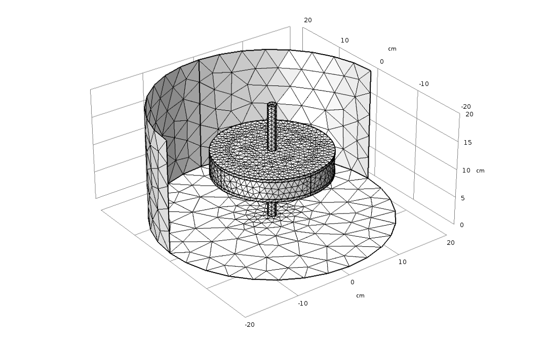 A geometry built in centimeters where the units are now shown on the axes.
Option for Switching Off Mesh Rendering
A new button in the Graphics toolbar enables you to switch off the rendering of the mesh. This makes it easier to see the interior of a 3D object, regardless of which part of the geometry has a mesh.

New button in the Graphics toolbar for switching on/off the rendering of the mesh.
Preview Evaluation Plane Functionality for Far-Field and Directivity Plots
You can now use the Preview Evaluation Plane feature in far-field and directivity plots. This plots the circle (scaled) where the far-field evaluation is carried out, as well as the evaluation plane normal and reference direction vectors (the direction that represents 0 degrees in polar plots). This greatly helps to visualize and verify that the evaluation is carried out at the correct location after entering or modifying the evaluation settings.
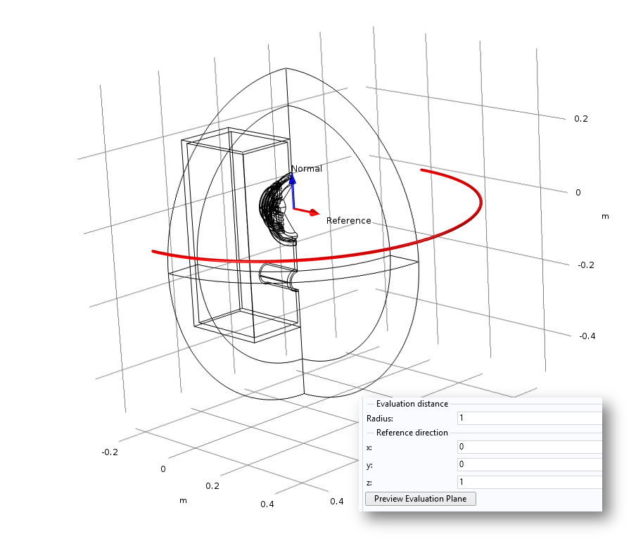 The preview evaluation plane and the plane's normal and reference directions for far-field plots with its corresponding settings. From the Loudspeaker Driver in a Vented Enclosure model.
Application Library path for an example that shows the preview evaluation plane:
Acoustics_Module/Electroacoustic_Transducers/vented_loudspeaker_enclosure