Wave Optics Module Updates
For users of the Wave Optics Module, COMSOL Multiphysics® version 5.3 brings new variables for postprocessing far-field radiation patterns, new default settings to improve your modeling experience, and a new Fresnel Lens tutorial model. Review all of the Wave Optics Module updates in more detail below.
New Far-Field Postprocessing Variables
Additional postprocessing variables have been added to the physics interfaces that calculate far-field radiation patterns. The previous gain variable is clarified with gain and realized gain by the input impedance mismatching factor. These postprocessing variables can be used in far-field plots to visualize the characteristics of an antenna.
- EIRP and EIRPdB: effective isotropic radiated power and its dB-scaled value
- gainEfar and gaindBEfar: gain excluding input mismatch and its dB-scaled value
- rGainEfar and rGaindBEfar: realized gain including input mismatch and its dB-scaled value
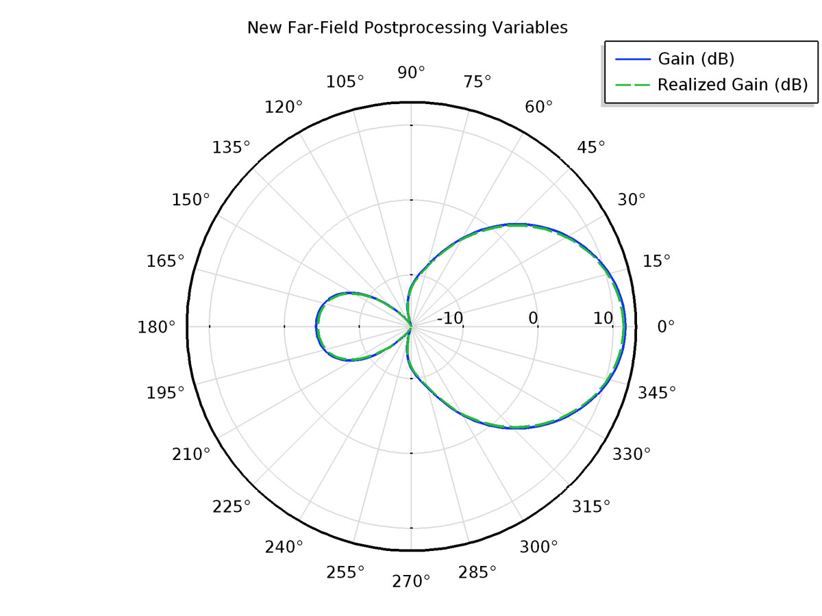
The far-field radiation gain and realized gain pattern on an xy-plane of a new Application Library example, a double-ridged horn antenna at 3 GHz.
Application Library path for the new far-field postprocessing variable: RF_Module/Antennas/double_ridged_horn_antenna
Surface Magnetic Current Density
The new Surface Magnetic Current Density boundary condition has been added to the Electromagnetic Waves, Frequency Domain interface and specifies a surface magnetic current density at both exterior and interior boundaries. Magnetic current density is described by a 3D vector. However, because it flows along a surface, it can be alternatively represented for more efficient modeling. To achieve this, the COMSOL Multiphysics® software projects this current density onto a boundary surface and neglects its normal component. The new boundary condition has been provided for special modeling situations, such as for modeling electric dipoles.
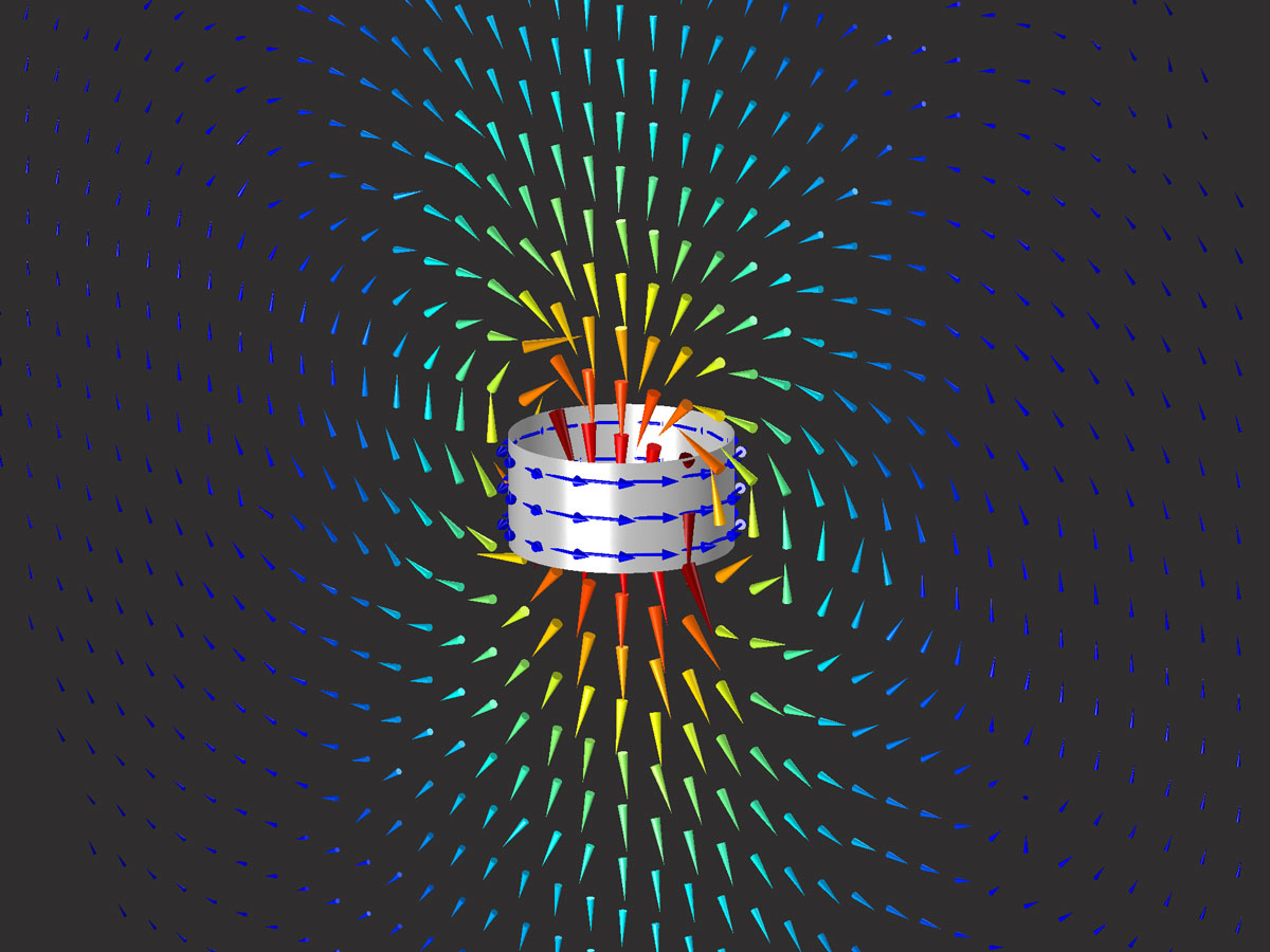
Surface magnetic current density (blue arrows) on a cylindrical coil through use of the Surface Magnetic Current Density boundary condition in the Electromagnetic Waves, Frequency Domain interface. The electric field pattern (cone) resembles that of a short dipole antenna.
New Default Settings for Enhanced Usability
Many default settings have been updated to reduce the number of modeling steps and enhance usability:
- Mesh reads the frequency or wavelength from study steps automatically for the Electromagnetic Wave, Frequency Domain interface
- Finer angular resolution (theta 45, phi 45) for the 3D far-field plot
- Automatic excitation is now turned on for the first port
- Eigenfrequency search method around shift is now set to Larger real part for Frequency-Domain Modal analyses
- The Linper operator is applied internally for excited ports and no longer needs to be specified by the user for Frequency-Domain Modal analyses
- The S-parameter descriptions have been simplified