CFD Module Updates
For users of the CFD Module, COMSOL Multiphysics® version 5.3 brings a new v2-f turbulence model for simulations over curved surfaces, an algebraic multigrid solver (AMG) that vastly improves solving CFD simulations, and automatic treatment of walls to provide high accuracy in turbulent flows. Browse these and more CFD Module updates and features below.
New Fluid Flow Interface for the v2-f Turbulence Model
The v2-f turbulence model, which is an extension of the k-ε turbulence model, provides highly accurate solutions for flows with strong turbulence anisotropy. An example of when to use this turbulence model over others is when flow occurs over curved surfaces, such as in the cyclone separator presented in the image. This model successfully captures the flow pattern, including the free vortex, which is inherently difficult in cyclone simulations and is largely impossible to perform with standard two-equation turbulence models.
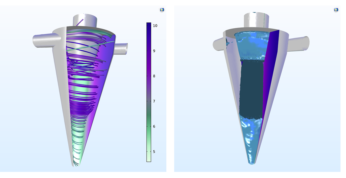 Streamlines and pressure field (left) and vortex core (right) in a model of the flow in a cyclone separator.
Application Gallery link:
Flow in a Hydrocyclone
Automatic Wall Treatment for Turbulent Flow
New functionality for wall-bounded turbulent flows allows for the automatic switching between a low Reynolds number turbulence model formulation and wall functions when solving your model. This functionality is available and is selected by default for the following turbulence models: Algebraic yPlus, L-VEL, k-ω, SST, Low Reynolds number k-ε, Spalart Allmaras, and v2-f.
If the mesh resolution close to the wall is adequate, then a low Reynolds formulation is used. Yet, when the mesh is too coarse, wall functions together with the selected turbulence model are automatically used instead. Switching between the two can occur in the same model. The functionality for automatically treating walls for turbulent flow provides the accuracy allowed by your mesh resolution, while also inheriting the robustness that is provided by wall functions.
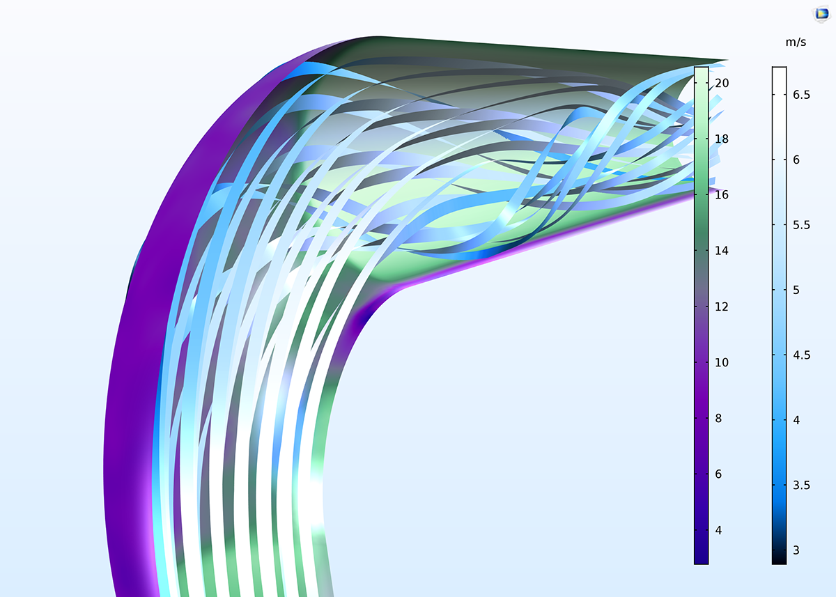 The wall's mesh resolution in viscous dimensionless units (color legend Aurora Borealis, in this figure) determines the functionality for automatically treating walls — either a low Reynolds turbulence model formulation or a wall function. The lower the value of the viscous dimensionless units, the higher the wall's mesh resolution and applicability for using a low Reynolds turbulence model formulation.
Application Library path for an example that uses automatic wall treatment:
CFD_Module/Single-Phase_Benchmarks/pipe_elbow
Automatic Translation Between Turbulence Models
A successful strategy for modeling turbulent flows is to start with a relatively simple turbulence model to gain an understanding of the system and for troubleshooting the model setup. Once you have a working model that gives reasonable results, a possible next step would be a more sophisticated — and maybe more computationally expensive — turbulence model for higher accuracy.
For this purpose, we have introduced a new functionality that "translates" the meaning of the turbulence variables from one turbulence model to another one. This means that you do not have to redefine the domain settings and boundary conditions for a second turbulence model. Additionally, you can use the existing solution as an initial condition for increased robustness and faster conversion in the solution of your second turbulence model problem.
Algebraic Multigrid (AMG) Solver for CFD
The smoothed aggregation algebraic multigrid (SA-AMG) method has been extended to work with the specialized smoothers for CFD in COMSOL Multiphysics®: SCGS, Vanka, and SOR Line.
Use of the alternative geometric multigrid (GMG) solver usually requires several mesh levels to be considered, which can create issues when trying to mesh and solve models with varying geometric details of different sizes. The SA-AMG solver only requires one mesh level, making the meshing process much easier and the solving process much more robust for large problems and "difficult" geometries.
For example, in the fluid-structure interaction model of a solar panel (in the image), the struts and beams supporting the panels are small in comparison to the air domain surrounding it. This difference in dimensions makes it difficult to efficiently mesh the air domain together with the smaller parts and components, which would be made even more difficult if three meshes of different sizes are to be created. The SA-AMG solver requires only one mesh level, which is far easier to obtain.
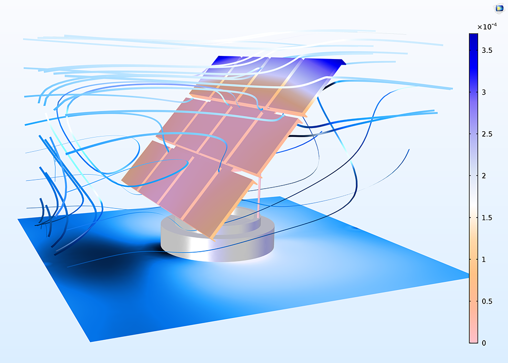
Fluid flow past a solar panel and the pressure distribution on the surface of it undergoing fluid-structure interaction behavior. The difference in the dimensional sizes of the supporting struts and beams against the surrounding air domain leads to challenges when meshing the model. With the SA-AMG solver, only one mesh level is required for the solution process, which is far faster and easier to achieve compared to the solution process with the GMG solver, which requires three mesh levels.
Application Library paths for examples that use the AMG Solver for CFD:
CFD_Module/Single-Phase_Benchmarks/ahmed_body
CFD_Module/Nonisothermal_Flow/displacement_ventilation
New Formulation and Tutorials for High-Mach Number Flow
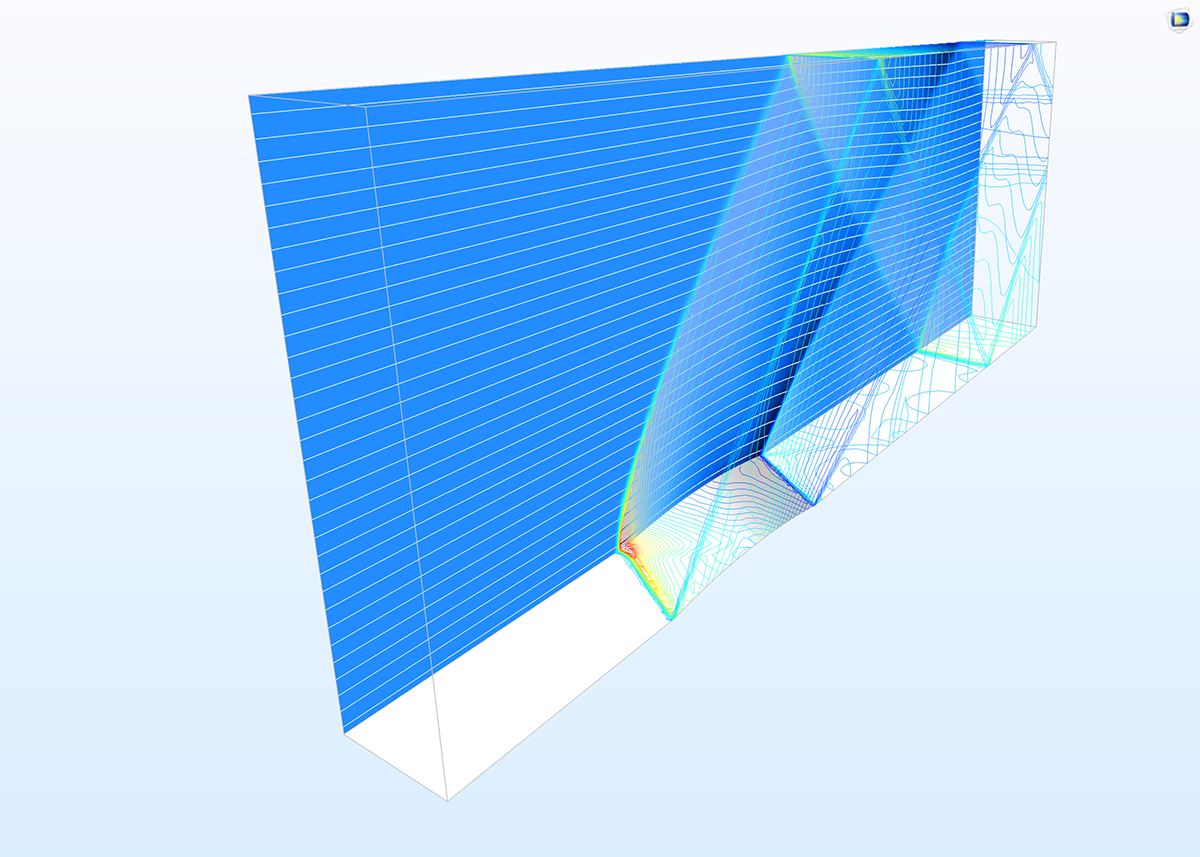
The High-Mach Number Flow interface combines the momentum equations with the energy equations for inviscid flows close to or above Mach 1. This has now been improved for better accuracy through developing a formulation of the momentum equations. In addition, three new tutorial models illustrating supersonic flows are introduced in the Application Library: The Euler Bump 3D, Expansion Fan, and Supersonic Ejector tutorials. These examples all reproduce results from scientific studies.
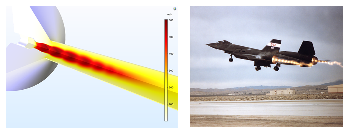 Shock diamonds in the velocity field of supersonic flow from a supersonic ejector model (left). Shock diamonds behind the engines of an SR-71 jet (right); image credit: NASA. NASA does not endorse the COMSOL Multiphysics® software.
Application Library path for the new High-Mach Number Flow tutorials:
CFD_Module/High_Mach_Number_Flow/euler_bump
CFD_Module/High_Mach_Number_Flow/expansion_fan
CFD_Module/High_Mach_Number_Flow/supersonic_ejector
New Interior Wall Boundary Condition
The Darcy's Law, Richards Equations, and Two-Phase Darcy's Law interfaces can now define thin interior walls. The Interior Wall feature is useful to avoid meshing thin impermeable structures embedded in porous media, such as retaining walls, plates, slabs, etc., thus reducing computational time and resources.
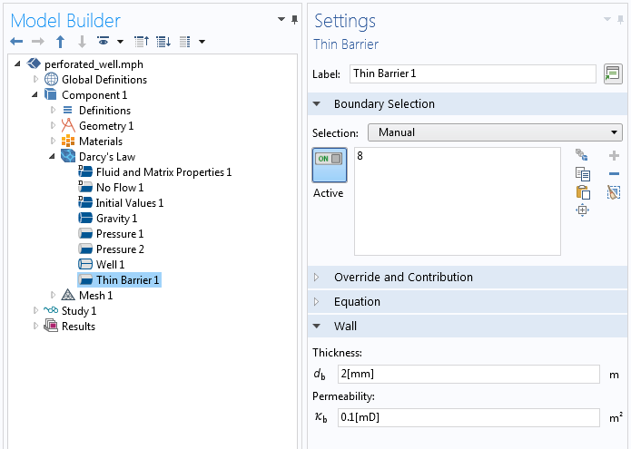
New Thin Barrier Boundary Condition
In the Darcy's Law and Richards Equations interfaces, you can now define permeable walls on interior boundaries with the Thin Barrier boundary condition. These internal boundaries are typically used to represent thin, low-permeability structures. With the Thin Barrier boundary condition, you avoid meshing thin structures like geotextiles or perforated plates, thus reducing computational time and resources.
New Tutorial: Helmholtz Resonator with Flow, Interaction of Flow and Acoustics
Helmholtz resonators are used in exhaust systems, as they can attenuate a specific narrow frequency band. The presence of a flow in the system alters the acoustic properties of the resonator and the transmission loss of the subsystem. In this tutorial model, a Helmholtz resonator is located as a side branch to a main duct. The transmission loss through the main duct is investigated when a flow is introduced.
The mean flow is calculated with the SST turbulence model for Ma = 0.05 and Ma = 0.1. The acoustic problem is then solved using the Linearized Navier-Stokes, Frequency Domain (LNS) interface. The mean flow velocity, pressure, and turbulent viscosity are coupled to the LNS model. Results are compared to measurements found in a journal paper and the amplitudes and resonance locations show good agreement with the measurement data (as seen in the 1D plot). The balance between attenuation and flow effects needs to be modeled rigorously in order for the resonance location to be correct.
Note: This model requires both the Acoustics Module and the CFD Module.
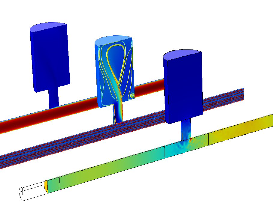 Acoustic sound pressure level distribution (front), surface streamlines (middle), and the background flow velocity amplitude (back) in a Helmholtz resonator located as a side branch to a main duct.
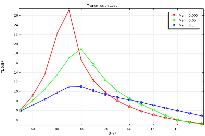 Transmission loss calculated using the LNS model for three flow configurations.
Application Library path:
Acoustics_Module/Aeroacoustics_and_Noise/helmholtz_resonator_with_flow
New Reacting Flow in Porous Media Interface
Modeling packed beds, monolithic reactors, and other catalytic heterogeneous reactors is substantially simplified with the new Reacting Flow in Porous Media multiphysics interface. This defines the diffusion, convection, migration, and reaction of chemical species for porous media flow, without having to set up separate interfaces and couple them. The multiphysics interface automatically combines all of the couplings and physics interfaces required for the modeling of heterogeneous catalysis together with porous media flow and dilute or concentrated chemical species transport.
As this multiphysics interface complements similar ones for laminar and turbulent flow, you can switch or define new couplings to other types of flow models without having to redefine and set up a new interface for the participating physical phenomena. The Settings window allows you to select the type of flow to be modeled as well as the transport of chemical species, without losing any of the defined material properties or reaction kinetics. This means that you can compare different reactor structures or model flow in both free and porous media in one reactor, even when the two regimes are connected (see image).
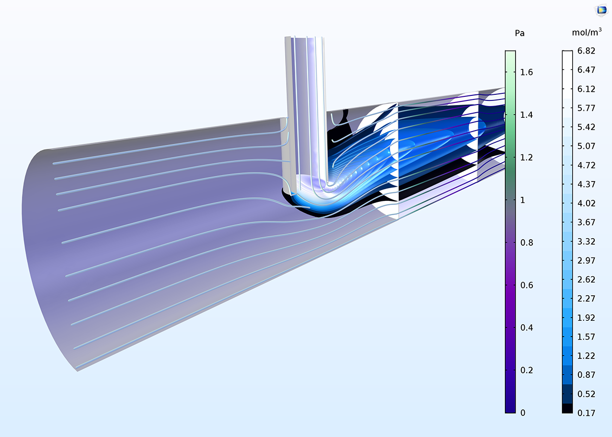
Model of a porous microreactor showing the concentration isosurfaces of a reactant injected through a vertical needle into a free flow containing a second reactant that is then forced through a monolithic catalytic porous media section of the reactor. The model can now be fully defined with the new Reacting Flow in Porous Media multiphysics interface.
Application Library path for an example using the new Reacting Flow in Porous Media interface:
Chemical_Reaction_Engineering_Module/Reactors_with_PorousCatalyst_porous_reactor
New Transport of Diluted Species in Fractures Interface
Fractures have thicknesses that are very small compared to their length and width dimensions. It is often difficult to model the transport of chemical species in such fractures through having to mesh the thickness of the fracture surface, due to the aspect ratios brought about by the large differences in size dimensions. The new Transport of Diluted Species in Fractures interface treats the fracture as a shell, where only the transverse dimensions are meshed as a surface mesh.
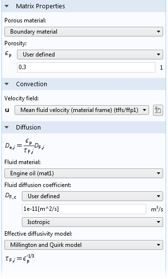
The interface allows you to define the average fracture thickness, as well as the porosity in cases where the fracture is considered to be a porous structure. For the transport of the chemical species, the interface allows definition of effective diffusivity models to include the effects of porosity. Convective transport can be coupled to a Thin-Film Flow interface or through including your own equations to define fluid flow through the fracture. Additionally, chemical reactions can be defined to occur within the fractures, at its surfaces, or in a porous medium that encompasses the fracture.
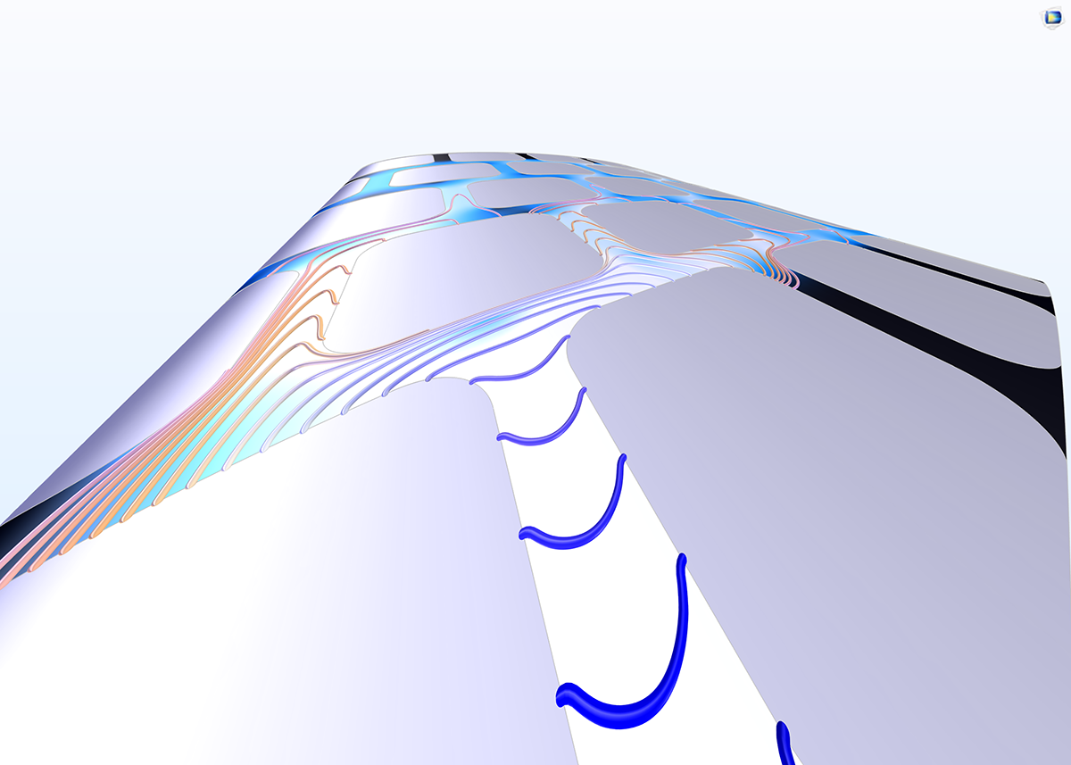 Transport of diluted species along a slightly curved fracture surface. The curved surface consists of an imprinted tortuous path through the surface where flow and chemical species transport occur.
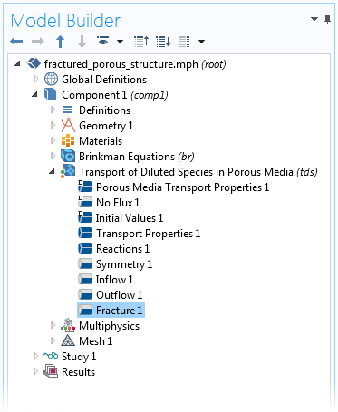
Fracture Surfaces in the Transport of Diluted Species in Porous Media Interface
In cases where transport occurs in a fractured, porous 3D structure, the new Fracture boundary condition lets you model transport in the thin fractures without having to mesh them as 3D entities. The Fracture boundary condition is included in the Transport of Diluted Species in Porous Media interface (see image) and has the same settings as in the Transport of Diluted Species in Fractures interface (described above). Fluid flow and chemical species transport are seamlessly coupled between a 3D porous media structure and fluid flow and chemical species transport in a fracture.
The image below shows the concentration field in a porous reactor model. In the model, a twisted fracture "leaks" reactants deeper into the porous catalyst, from left to right, at a faster rate than the transport through the porous media. This is because the fracture surface has a much higher average porosity compared to the surrounding porous catalyst, which gives a higher mass transport rate.
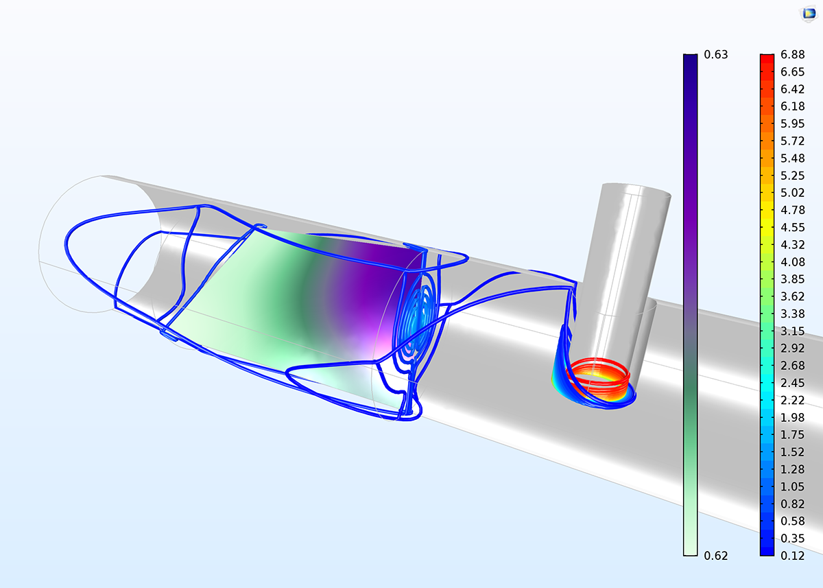 Concentration contours through the 3D reactor and surface concentration in the fracture surface. The higher mass transport rate in the fracture surface gives a larger penetration (from right to left) of unreacted species into the catalyst bed. We can see that the change in concentration from right to left is very small in the fracture surface (from 0.63 to 0.62 mol/m3).