Particle Tracing Module Updates
For users of the Particle Tracing Module, COMSOL Multiphysics® version 5.3 includes many new features, highlighted by the Periodic Condition and Rotating Frame features for particle tracing in sectors and rotating machinery, respectively. Additionally, you can define random initial positions for particle releases and visualize particle paths as ribbons. Browse all of the new features and functionality in the Particle Tracing Module below.
Particle Tracing Periodic Condition
You can use the new Periodic Condition feature to model particle tracing in periodic structures or in geometries with sector symmetries. When a particle reaches a surface with the Periodic Condition, it is immediately mapped to a destination point on a second surface. After the particle is mapped to the destination surface, its velocity can either be kept the same, rotated (for sector symmetry), or set to a new value by a user-defined expression.
Particles, colored by their unique particle index, traveling through a domain with sector symmetry.
Rotating Frames
The Rotating Frame feature in particle tracing is now available for rotating frames of reference. When you specify the center of rotation, direction of rotation, and angular velocity magnitude of the frame, the centrifugal, Coriolis, and Euler forces that are exerted on the particles are automatically applied. Particle tracing in rotating frames allows for easier modeling of particle motion in rotating machinery, such as mixers and turbomolecular pumps, because the particle trajectories can be computed in a frame of reference that is attached to the moving geometry.
By adding this feature to a model, release-based features will include an option to specify whether the initial particle velocity is defined with respect to the rotating frame or with respect to the inertial (nonrotating) frame. This latter additional feature is activated in the Advanced Settings section by selecting the Subtract moving frame velocity from initial particle velocity check box.
Particles are released at rest with respect to the rotating frame of reference; that is, they have a nonzero initial velocity with respect to a nonrotating (inertial) frame. Due to the fictitious centrifugal and Coriolis forces, the particles spiral out toward the boundary.
Particles are released at rest with respect to the nonrotating (inertial) frame of reference; that is, the frame velocity is subtracted from the initial velocity in the rotating (noninertial) frame. As a result, the balance of centrifugal and Coriolis forces causes the particles to orbit the center of rotation at constant speed.
Application Library path for an example showing the Rotating Frame feature:
Particle_Tracing_Module/Tutorials/turbomolecular_pump
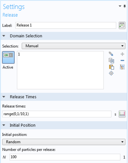
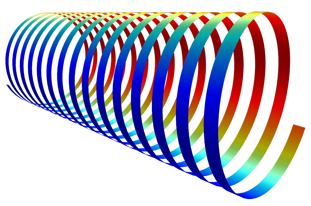
Random Initial Positions
You can now release particles at random initial positions on selected domains, boundaries, and edges. Unique positions are chosen for each release time. This is available in the Release, Inlet, and Release from Edge features.
Particles are released at random positions on an Inlet boundary and are carried through a cylindrical pipe. The color expression is proportional to the release time.
Ribbons on Particle Trajectories
You can now visualize particle trajectories as ribbons. Unlike with lines and tubes, plotting the particle trajectories as ribbons gives you the flexibility to specify an orientation as well as a path for the particle motion. For curved trajectories, it is useful to use built-in expressions for the normal and binormal directions to better visualize the particle motion.
Motion of a charged particle in a uniform magnetic field. The ribbon has been oriented so that it is parallel with the binormal direction for the curved trajectory.
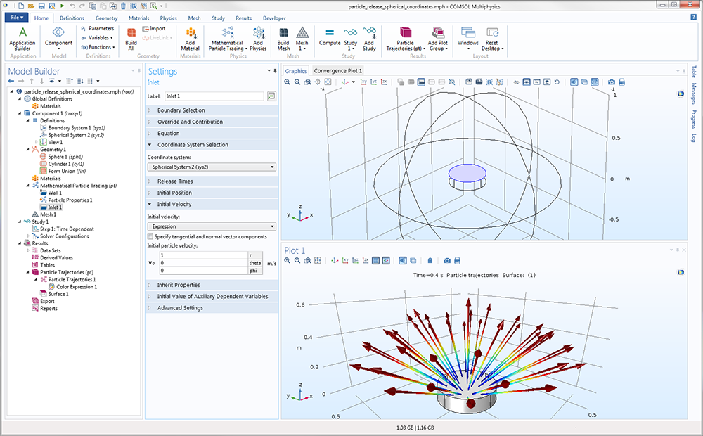
Coordinate System Selection for Inlets
When releasing particles at a boundary using the Inlet feature, you can initialize the particle velocity or momentum using any coordinate system that has been defined for the model component.
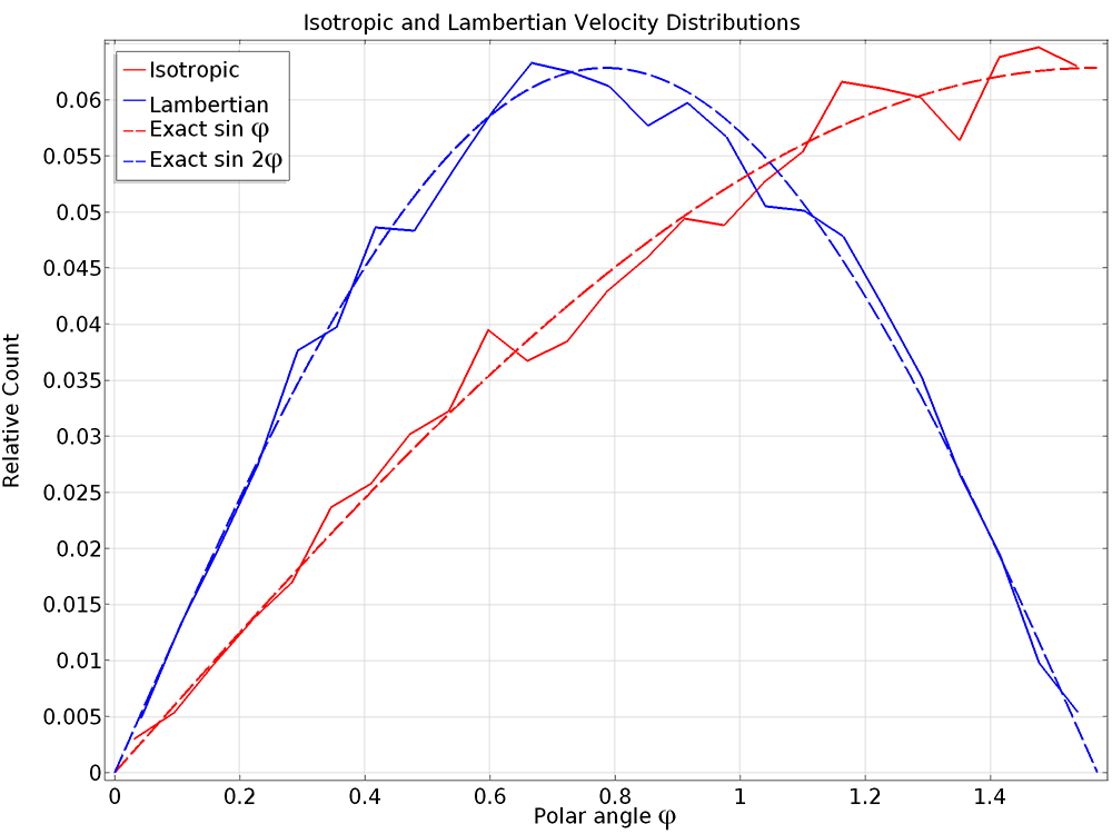
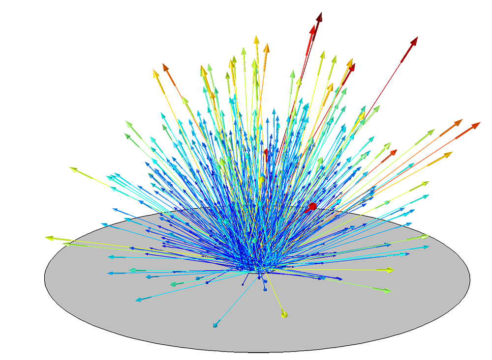
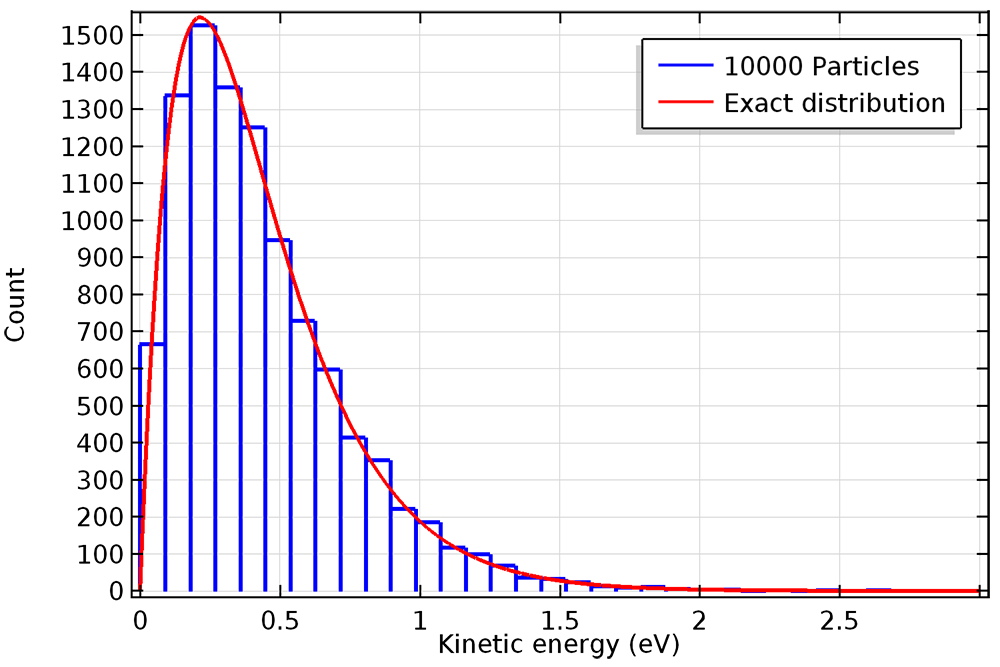
Lambertian Velocity Distribution
The particle release features now include an option to release particles with a Lambertian velocity distribution in 3D. Particles are released with initial directions based on Lambert's cosine law, also known as Knudsen's cosine law in molecular dynamics.
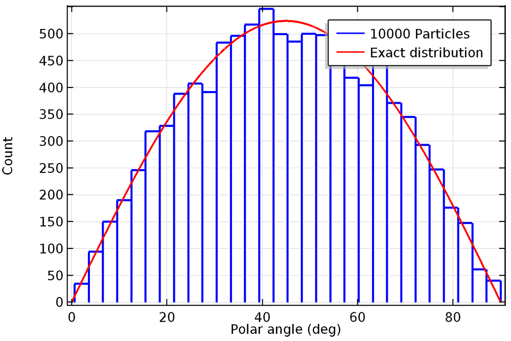
Lambert's cosine law states that the probability that a particle will be released through a differential solid angle element dω with polar angle θ is proportional to cos θ. By comparison, in the isotropic hemispherical distribution, the particle is equally likely to be released through any differential solid angle in the hemisphere.
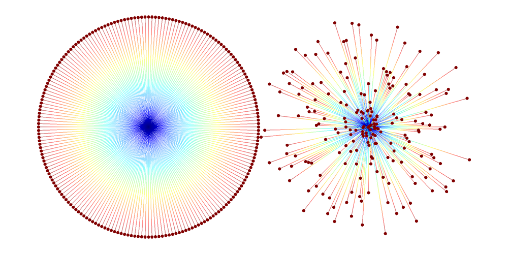
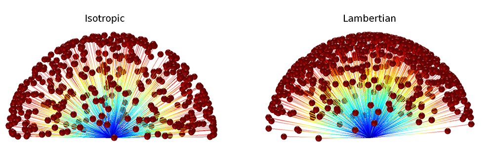 Comparison of particle distributions in an isotropic hemispherical release (left) and a Lambertian release (right). The Lambertian release more heavily favors directions closer to the hemisphere axis.
Nonuniform Magnitudes in Velocity Distributions
For the spherical, hemispherical, conical, and Lambertian velocity distributions, it is now possible to release particles with a distribution of speeds as well as directions.
By default, every particle that is released from the same point in a velocity distribution will have the same magnitude. However, by expressing the initial speed in terms of the unique particle index, you can apply a different initial speed to each particle without changing the distribution of particle directions. This makes it easier to include distributions of particle speed or energy, as well as direction.
Particles with uniform speed (left) or a pseudorandom distribution of different speeds (right). The distribution of particle velocity directions has been left unchanged; it is an isotropic circle for both releases.
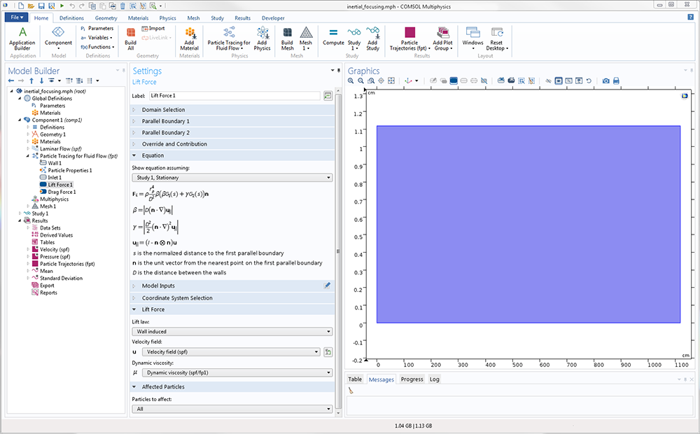
Lift Force
A dedicated Lift Force feature is now available for the Particle Tracing for Fluid Flow interface. Lift forces are relevant when particles move in a nonuniform fluid velocity field. The drag force acts in parallel with the fluid velocity with respect to the particle, whereas the lift force typically acts normal to it.
Two different formulations of the lift force are available: Saffman and Wall induced. The Saffman formulation for lift force is applicable to inertial particles in a shear flow that are an appreciable distance away from boundaries. The specialized Wall induced formulation is available for neutrally buoyant particles in channels.
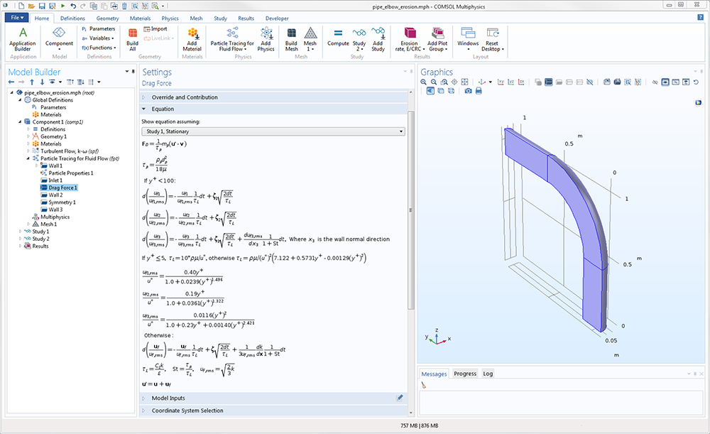
Anisotropic Turbulent Dispersion
When applying a random turbulent dispersion term to the drag force on particles in a fluid using the continuous random walk model, the turbulent dispersion can now be either isotropic (the default) or anisotropic. If anisotropic turbulence is used, the turbulent dispersion terms are computed using specific expressions for the streamwise, spanwise, and wall normal directions. Anisotropic turbulence can provide a more realistic depiction of particle motion in a turbulent flow when the particles are close to walls.
Thermionic Emission of Electrons
A dedicated Thermionic Emission feature is now available to model the release of electrons from a hot metal cathode and is available in the Charged Particle Tracing interface. The total current density released from the boundary is computed using Richardson's law, where the effective Richardson constant, work function of the metal, and temperature can be specified.
 Thermionic emission of electrons from a boundary. The color expression is proportional to the kinetic energy of the electrons.
Application Library path for an example showing the Thermionic Emission feature:
Particle_Tracing_Module/Charged_Particle_Tracing/planar_diode
Drag Correction Factor for Particles Close to Walls
A new drag correction factor adjusts the drag force that particles experience as they approach walls. Most common drag laws, such as the Stokes drag law, are formulated under the assumption that the particle is extremely small relative to the geometry size. These wall corrections improve the accuracy when the ratio of the particle radius to the distance to the nearest wall is not negligibly small. Simply select the Include wall corrections check box to enable these corrections.
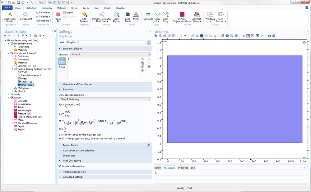
Settings window for the Drag Force feature with the Include wall corrections option selected so as to account for nearby walls.
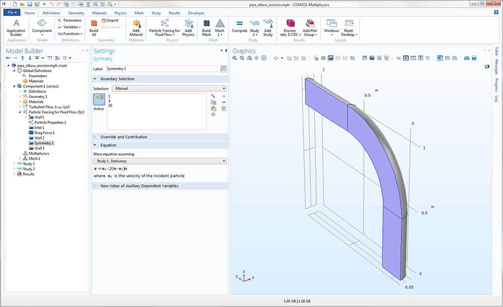
Symmetry Condition for Particle Tracing
The specialized Symmetry boundary condition is now available in the Charged Particle Tracing and Particle Tracing for Fluid Flow interfaces, and reduces the size of your model and computational resources required to solve it. It is a useful and special case of the Wall boundary condition that always imposes model particles to be specularly reflected at the boundary. This means that for every particle that would leave the modeling domain through a symmetry plane, an identical particle would simultaneously enter the modeling domain at the same location and same time.
Extra Time Steps in Trajectory Plots
When plotting particle trajectories, it is now easier than ever to plot additional time steps that correspond to particle-wall interaction times. The number of these extra time steps can now be controlled directly from the Settings window for the Particle Trajectories plot. Built-in options are available to specify the maximum number of extra time steps directly or as a multiple of the number of stored solution times.
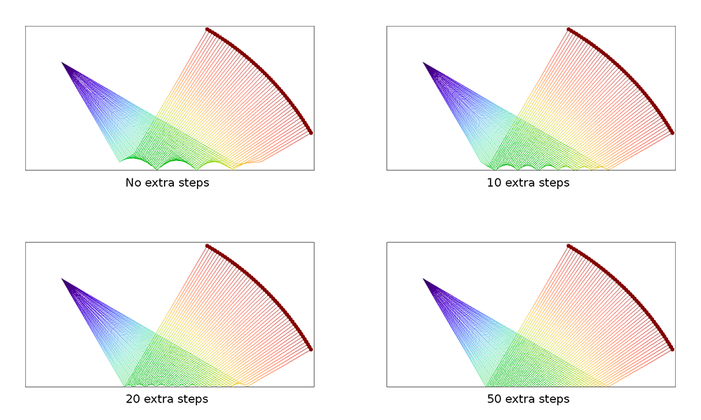 As the number of extra time steps in the trajectory plot is increased, the times at which each particle bounces off the wall can be seen more clearly.
New Options for Inlet Pairs
When releasing particles from an inlet pair defined on an assembly, you can now choose to release the particles from only the source boundary, the destination boundary, or both. This is most noticeable when using a mesh-based release of particles, since the mesh on either side of the identity pair can be different.
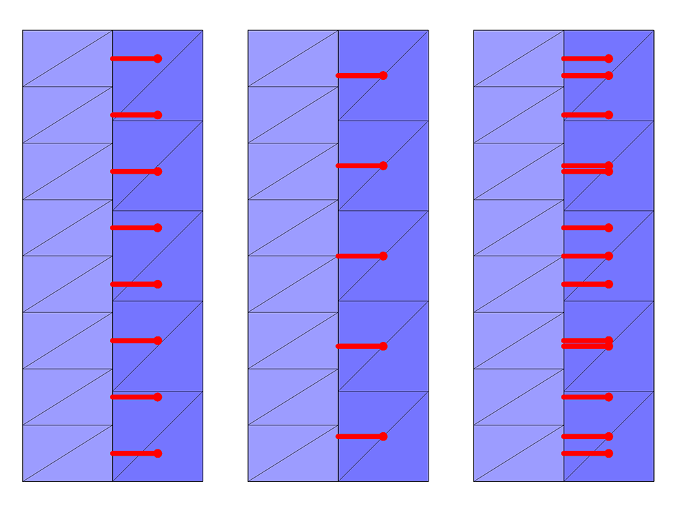
Mesh-based release of particles from the source boundary (left), the destination boundary (middle), or both source and destination (right). In each rectangle, the source boundary is on the side of the lighter-colored mesh.
Alternative Way to Assign Weights in Bidirectionally Coupled Space Charge Models
When using the Bidirectionally Coupled Particle Tracing study step to model electric particle-field interactions, it is now possible to assign different weights to the space charge density computed during different iterations of the solver loop. There are built-in options to make these weights remain constant (the default) or increase them in an arithmetic or geometric sequence. This can lead to faster convergence of bidirectionally coupled models in which the electric field and the trajectories of charged particles strongly influence each other.
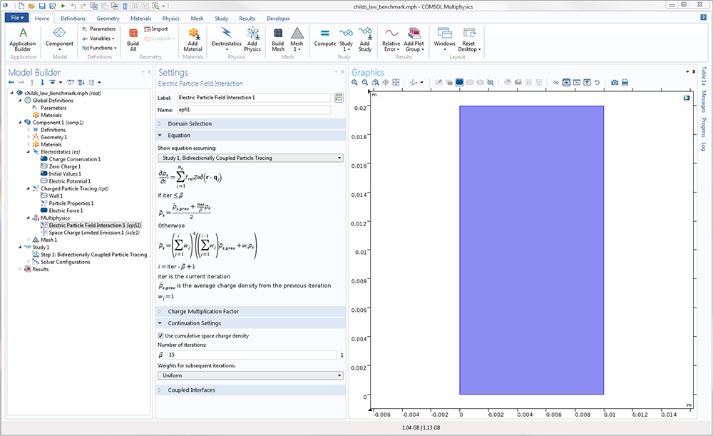
The weights for the space charge density in each iteration of the Bidirectionally Coupled Particle Tracing study can be uniform, an arithmetic sequence (shown above), or a geometric sequence.
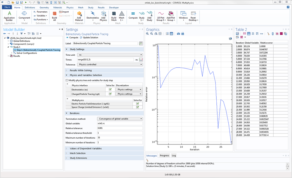
Convergence-Based Termination Criteria for Bidirectionally Coupled Models
For models that use the Bidirectionally Coupled Particle Tracing study step to iterate between stationary and time-dependent solutions, it is now possible to terminate the solver loop based on a convergence criterion instead of a fixed number of iterations. For example, when modeling bidirectionally coupled particle-field interactions, you can terminate the study when the relative error in the electron or ion current is sufficiently small. This allows you to state the level of accuracy you want, without having to expend computational resources to complete a fixed number of iterations after this criterion is satisfied.
New Component Couplings on Particles
New component couplings are automatically created for each instance of a particle tracing interface, and the behavior of the old component couplings has changed. The old component couplings, for example, pt.ptop1(expr), now automatically exclude both particles that have not yet been released and particles that have disappeared. The degrees of freedom of such particles are usually not-a-number (NaN), so it is convenient to automatically exclude them when evaluating sums and averages over the totality of particles.
The following table lists the component couplings that are automatically created for the Mathematical Particle Tracing interface.
| Name | Description |
|---|---|
| `pt.ptop1(expr)` | Sum of expression `expr` over active, stuck, and frozen particles |
| `pt.ptop_all1(expr)` | Sum of expression `expr` over all particles |
| `pt.ptaveop1(expr)` | Average of expression `expr` over active, stuck, and frozen particles |
| `pt.ptaveop_all1(expr)` | Average of expression `expr` over all particles |
| `pt.ptmaxop1(expr)` | Maximum of expression `expr` over active, stuck, and frozen particles |
| `pt.ptmaxop_all1(expr)` | Maximum of expression `expr` over all particles |
| `pt.ptminop1(expr)` | Minimum of expression `expr` over active, stuck, and frozen particles |
| `pt.ptminop_all1(expr)` | Minimum of expression `expr` over all particles |
| `pt.ptmaxop1(expr, evalExpr)` | Evaluate `evalExpr` at the maximum of expression `expr` over active, stuck, and frozen particles |
| `pt.ptmaxop_all1(expr, evalExpr)` | Evaluate `evalExpr` at the maximum of expression `expr` over all particles |
| `pt.ptminop1(expr, evalExpr)` | Evaluate `evalExpr` at the minimum of expression `expr` over active, stuck, and frozen particles |
| `pt.ptminop_all1(expr, evalExpr)` | Evaluate `evalExpr` at the minimum of expression `expr` over all particles |
Additional Statistics Based on Particle Status
When the Store particle status data check box is selected, the following new variables will be defined.
(Note: The expressions are written for an instance of the Mathematical Particle Tracing interface with tag pt. Physics interface tags will naturally be different for different physics interfaces.)
| Tag | Name | Description |
|---|---|---|
| pt.fac | `pt.ptop1(pt.fs==1)` | Fraction of particles active at final time |
| pt.ffr | `pt.ptop1(pt.fs==2)` | Fraction of particles frozen at final time |
| pt.fst | `pt.ptop1(pt.fs==3)` | Fraction of particles stuck at final time |
| pt.fds | `pt.ptop1(pt.fs==4)` | Fraction of particles disappeared at final time |
| pt.fse | `pt.ptop1(!primary&&pt.fs>0)/pt.Ms` | Fraction of secondary particles released at final time |
New Tutorial: Inertial Focusing Benchmark
For more than 50 years, it has been known that neutrally buoyant particles in a flow channel tend to converge to specific locations in the channel cross section. For a cylindrical pipe, or two parallel planes carrying a Poiseuille flow, the equilibrium position is about 0.6 times the pipe radius, or a distance from the parallel walls of about 0.2 times the channel width, respectively. This is sometimes called the Segre-Silberberg effect, while a ring of particles with a radius of 0.6 times the pipe radius is sometimes called the Segre-Silberberg annulus.
In this benchmark model, we reproduce the case of a flow channel bounded by two parallel walls. Wall-dependent lift and drag forces are exerted on the neutrally buoyant particles as they are carried along the channel by a parabolic fluid velocity profile. As particles are carried through the channel, the inertial lift force causes them to reach equilibrium positions at distances from the center of 0.3D, where D is the distance between the walls. These equilibrium positions are consistent with the Segre-Silberberg effect.
Particle trajectories in a rectangular channel. The color expression is the y-component of the particle velocity. Note that the channel is scaled for easier viewing, but actually has a 1000-to-1 aspect ratio.
Application Library path:
Particle_Tracing_Module/Fluid_Flow/inertial_focusing
New Tutorial: Thermionic Emission in a Planar Diode
When electrons are emitted from a heated cathode in a plane parallel vacuum diode, they contribute to the space charge density in the diode, which in turn affects the electric potential distribution. If the potential difference between the cathode and the anode is not sufficiently large, a potential minimum forms between them, repelling electrons of insufficient energy back toward the cathode. Such a diode is said to be operating in the space charge limited regime.
In this benchmark model, the dedicated Thermionic Emission feature is used to release thermal electrons from a cathode of a specified temperature and work function. The electron trajectories are bidirectionally coupled to the electric potential calculation in the diode using the specialized Electric Particle Field Interaction multiphysics coupling and Bidirectionally Coupled Particle Tracing study step. The electric potential distribution and the anode current compare favorably to the results of the analytical Langmuir-Fry model.

Electric potential close to the cathode in a planar diode, as compared to reference data. When self-consistent particle-field interactions are included in the model, a potential barrier forms next to the cathode.
Application Library path:
Particle_Tracing_Module/Charged_Particle_Tracing/planar_diode
New Tutorial: Einzel Lens
An Einzel lens is an electrostatic device used for focusing charged particle beams. It may be found in cathode ray tubes, ion beam and electron beam experiments, and in ion propulsion systems. This particular model consists of three axially aligned cylinders. The outer cylinders are grounded, while the cylinder in the middle is held at a fixed voltage. The 3D electrostatic field is computed with the Electrostatics interface and the particle trajectories are computed using the Charged Particle Tracing interface.
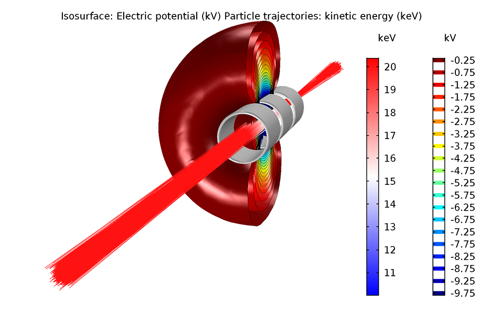 Electron trajectories in an Einzel lens. The beam is focused near the electrodes around which the isosurfaces of electric potential are shown.
Application Library path:
Particle_Tracing_Module/Charged_Particle_Tracing/einzel_lens
New Tutorial: Turbomolecular Pump
The Free Molecular Flow interface (available in the Molecular Flow Module) is an efficient tool for modeling extremely rarefied gases when the gas molecules move much faster than any geometric entities in the domain. For turbomolecular pumps, in which the blades move at speeds comparable to the thermal speed of the gas molecules, a Monte Carlo approach is needed.
In this example, the trajectories of gas molecules are computed in the empty space between two rotating blades of a turbomolecular pump. The model uses the new Rotating Frame feature that applies centrifugal and Coriolis forces to the particles, allowing the trajectories to be computed in a noninertial frame of reference that moves with the rotating blades. The effect of the blade velocity on the compression factor is shown using a Parametric Sweep.
Note: The model in the example also requires the Molecular Flow Module.
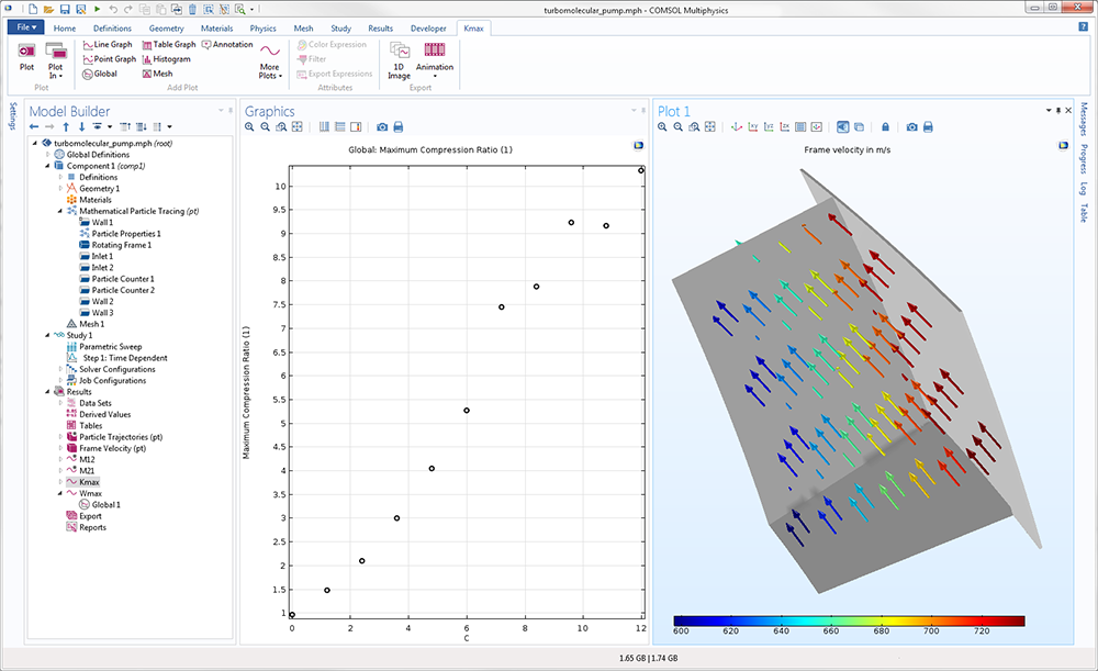
Screenshot of the Turbomolecular Pump tutorial model. As the blade velocity increases, molecules have a higher probability of being transmitted forward through the pump and a lower probability to be transmitted backward, as shown by the increasing compression ratio.
Application Library path:
Particle_Tracing_Module/Tutorials/turbomolecular_pump