

In the Application Builder, included with COMSOL Multiphysics version 5.2, the new Editor Tools window makes it possible to create simulation apps with a lot fewer clicks of the mouse. In this blog post, we will demonstrate how to create an app with Editor Tools using a simple simulation example, as well as show how to perform common user interface creation tasks more easily.
Introducing Editor Tools
While using the Application Builder in COMSOL Multiphysics version 5.2, you will quickly realize the usefulness of the new Editor Tools window, which allows you to insert groups of associated user interface components into your app more quickly. For example, when you want to use a model parameter as an input in your simulation app, using Editor Tools will not only give you an input field, but you will also get an associated text label with the parameter’s description and the proper unit label.
Let’s take a look at some common operations that you typically perform at the start of the app design process, which now require a lot fewer steps with the use of Editor Tools. In fact, if your goal is just to create simple apps, then Editor Tools may even be all that you need.
Expanding on a Flow Simulation App
Consider the following user interface of this deliberately oversimplified app for simulating the transient flow around a cylindrical object in a channel.

The magnitude of the velocity in a simulation of flow around a cylinder in a channel, where the cylinder is placed in the center.
The app is built on the Flow Past a Cylinder tutorial model that is available in the Application Library of the core COMSOL Multiphysics product. The only deviation from the Application Library tutorial model is that we have made a parameter available for the y-position of the cylinder.
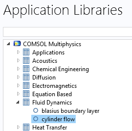
The cylinder flow model used as a basis for the example in this blog post.
The flow comes in from the left part of the channel, passes by the obstacle, and exits to the right. The app allows you to change the y-position of the cylinder and then recompute. The picture below shows the flow when the y-position is changed from 0.2 to 0.3 meters relative to the background coordinate system.

Flow around a cylinder in a channel where the cylinder is offset by 0.1 m.
In this case, the simulation takes about one minute on a standard workstation. However, if we go from a 2D simulation to a 3D case, the simulation time will increase, and then we can see an obvious shortcoming with the current design of the app’s user interface: previewing the geometry for the new obstacle position before recomputing. For this, we need a Plot Geometry button. Let’s now see how we can add a button with the new Editor Tools window.
You access the Editor Tools window by clicking on the corresponding button to the left in the ribbon of the Application Builder.
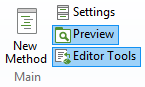
The new Editor Tools option in the Application Builder ribbon.
Adding a Plot Geometry Button
Now, navigate to the Geometry node in the tree of the Editor Tools window. Right-clicking on the node gives you two main options: Graphics and Button. (There is also a third option, Edit Node, which takes you back to the Model Builder tree for changing the contents of the node.) The first option, Graphics, will add a new graphics object for geometry visualization. However, in this case, we will select the second option, Button, which will reuse the existing graphics object for plotting the geometry.
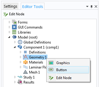
Selecting a Button in the new Editor Tools window.
In the Form Editor, we can drag and drop the new button object and, for example, place it to the left of the Compute button.
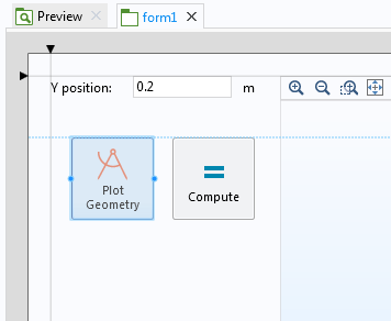
Positioning a button used to plot the geometry in the Form Editor.
If we look at the Settings window for the Plot Geometry button, we can see that Editor Tools automatically made a number of choices for us that we otherwise would have had to do manually:
- The button’s Text field is filled out with the text string: Plot Geometry.
- The built-in image file geometry_32.png was chosen as the icon, or Picture, for the button. The suffix 32 means that it is a 32-by-32 pixel image file.
- The Size of the button was changed from the default Small to Large.
- A command, Plot Geometry, was added to the command sequence.
- The input argument to the plot command was chose to be graphics1, allowing us to reuse the existing graphics object and thereby save room in the user interface.
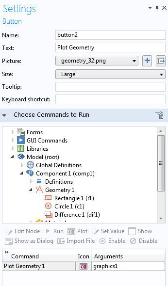
The settings window for the Plot Geometry button.
To put this in perspective, in order to perform all of these steps manually, we would start by selecting Button from the Insert Object menu in the ribbon and then continue by editing the Settings window according to the list above. If we would like to create a fully customized button, then we would have to specify all of the details manually.
We can now easily preview the geometry before solving.

The Plot Geometry button is used to preview the geometry for a cylinder with a y-displacement of 0.1 m.
Adding an Input Field
Using Editor Tools, we can easily add other types of form objects. In the model that is used as a basis for the app, there is a parameter for the inflow velocity. Locating it in the Editor Tools window and right-clicking on its node gives us two options: Input and Output.
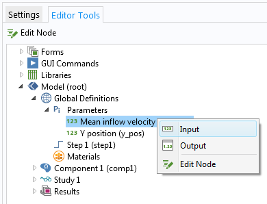
Adding an input field is made easy with Editor Tools.
Selecting Input followed by rearranging objects in the Form Editor gives us the following layout.
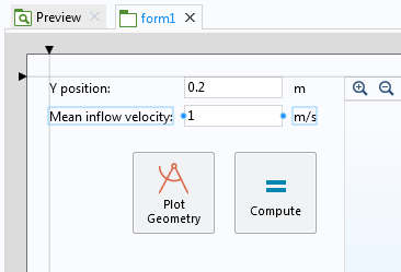
Using Editor Tools not only adds the input field but also a text label, Mean inflow velocity, and a unit, m/s. Again, such an approach automates a number of manual steps.
If we run the app and increase the inflow velocity to 2 m/s, we can see that there are vortexes shed from behind the cylinder. This is an example of a Kármán vortex street.

A Kármán vortex street appears when increasing the mean velocity.
Accessing the Solution at Different Times
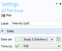
Let’s say that we would like the user to be able to access the velocity plot at different times. In the Model Builder, this is readily available as a drop-down list in the settings window of a plot node.
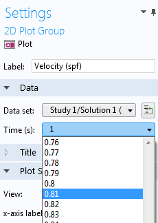
The Time drop-down list in the Velocity Plot node in the Model Builder.
However, if you try to add the option to your app user interface using Editor Tools, you will not find it. The reason is that there are hundreds of settings in the Model Builder that you may want to include in your user interface and, by default, they are not all visible. Making them all available would make the Editor Tools tree unnecessarily cluttered. Instead, you can selectively make such properties available by using another utility called Model Data Access. You will find this in the Model Builder, to the left in the ribbon.
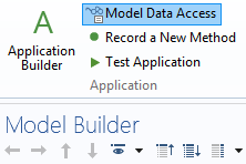
The Model Data Access button in the Model Builder.
Activating Model Data Access displays green check boxes next to the properties that you can make available to Editor Tools. Selecting the Time drop-down list will allow us to include this property in our user interface.
The Time drop-down list for the velocity plot with Model Data Access activated.
The Time property is now available in the Editor Tools tree under the Velocity node. We can right-click and select Input to get the corresponding list added to our user interface.
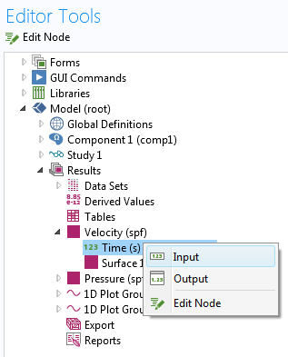
The Time list, as available from Editor Tools.
Finally, we can use Editor Tools to add a Plot button so that we can trigger a new visualization each time we select a new time. We can also use events to automatically trigger the plot — but we won’t discuss that approach here.
The final user interface is shown below.

We can, of course, easily expand this app with more functionality. It should be noted that Editor Tools can also be used together with the Method Editor for adding code corresponding to common operations.
In summary, Editor Tools is a great new utility with functionality right in between that of the Form Wizard and Insert Objects menu. When combined with Model Data Access, you can create sophisticated apps in very little time.
Application Examples
If you wish to see more elaborate examples, open and explore one of more than 60 application examples that are available in COMSOL Multiphysics version 5.2 (all add-on products are included). You will find these examples in the Applications folder in the Application Libraries of the add-on products. For example, the core product contains several example apps, including a new fluid app of a Helical Static Mixer.
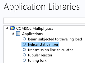
The location of the new Helical Static Mixer app example in the Application Libraries.

The Helical Static Mixer app with a visualization of the contact probability field.


Comments (2)
Adrian Quesada
March 20, 2019On the Flow Past a Cylinder tutorial model that is available in the Application Library of the core COMSOL Multiphysics product it has some particles for particles tracing, it is posible to add a botton to chose the amount of particles to be released on this tutorial?
Brianne Christopher
March 20, 2019Hello Adrian,
Thank you for your comment.
For questions related to your modeling, please contact our Support team.
Online Support Center: https://www.comsol.com/support
Email: support@comsol.com