When the German engineer F. H. Poetsch first developed the artificial ground freezing (AGF) method in 1883, he did so to avoid water within Belgian coal mines. The method, which first received praise in the late 1800s, remains similar to its original form and is still valuable today. To develop a more effective AGF method, we can turn to simulation analyses.
What Is the Artificial Ground Freezing Method?
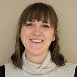
Artificial ground freezing is a construction technology that involves running an artificial refrigerant through pipes buried underground. As the refrigerant circulates through the pipe network, heat is removed from the ground and ice begins to form around the pipes. This in turn causes the soil to freeze. In other words, the process converts soil moisture into ice. Once the soil is frozen, it is both stronger (sometimes as hard as concrete) and has a greater resistance to water. This allows the soil to provide effective support to the relative infrastructures, particularly those that are larger and more complex.
Once frozen, soil becomes stronger and more resistant to water.
For the AGF method to be effective, we need to know the temperature distribution inside the system. Of the physical processes that occur in AGF, the most prominent is the phenomenon of transient heat conduction with phase change. Further, it is also important to consider the relationship between this phase change and the groundwater flow — particularly when there is a higher flow velocity. These elements can impact the development of the freezing wall and thus the strength and reliability of the AGF method.
To study the AGF method, a team of researchers from Hohai University turned to the COMSOL Multiphysics® software. Their case study involves using the method to strengthen soil at a metro tunnel entrance in Guangzhou, China.
Modeling the Artificial Ground Freezing Method and Groundwater Flow
For this specific example, the refrigerant that circulates throughout the pipe system is -30ºC brine. The subsurface temperature is reduced until the pore water is frozen and the freezing wall forms. The formation within the frozen area is made up of muddy sand, and the direction of the groundwater flow is primarily horizontal and normal in relation to the axial direction of the tunnel.
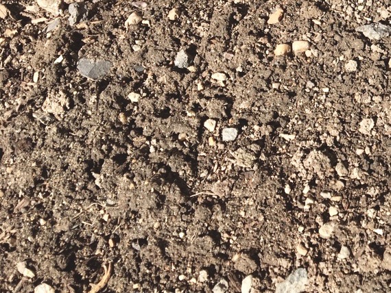
To simplify modeling heat transport in a saturated aquifer, the researchers used a 2D model based on a coupling of temperature and flow fields. The model, shown below, is 20 m in both length and height. Note that five monitoring points are included. These points are used to verify the accuracy of the model by comparing the calculated temperature results with in situ measurements.
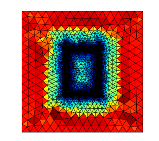
The AGF model’s geometry, with the monitoring points highlighted (left), and the model grid’s mesh (right). Images by Rui Hu and Quan Liu and taken from their COMSOL Conference 2016 Munich paper.
In this analysis, the following assumptions are made:
- The ice is incapable of moving and the medium cannot deform
- The aquifer is fully saturated, with a total porosity that remains constant
- The freezing point depression caused by solute concentrations is negligible
According to previous temperature monitoring data from the frozen area, there is an initial ground temperature of 15°C. The figure below shows the initial temperatures in various holes of thermal observation.
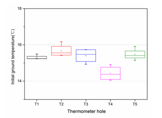
The initial temperatures in different holes for thermal observation. Image by Rui Hu and Quan Liu and taken from their COMSOL Conference 2016 Munich paper.
The cooling source of the freezing system is the lateral wall of the freezing pipe. Changes in the temperature of the lateral wall have the greatest impact on the temperature distribution within the system. It is possible to use the values from the temperature monitoring of the main pipe as approximations for the estimated temperature of the lateral wall. The plot below shows the fitting function and curve for the lateral wall temperature of the main pipe after a monitoring period of 40 days.
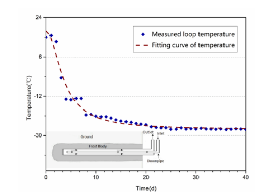
The fitting function and curve for the lateral wall temperature. Image by Rui Hu and Quan Liu and taken from their COMSOL Conference 2016 Munich paper.
With regards to groundwater flow, a flow velocity of 0.2 m/d is obtained via field tests. Between upstream and downstream, the head difference is calculated as 0.8 m.
Now onto the results. Let’s consider the temperature distribution and permeability coefficient for a range of times. In terms of temperature, when the freezing time increases, the cold temperature from the freezing pipes is primarily led downstream — with less of an influence upstream. The permeability coefficient results, which illustrate the formation of the freezing wall, indicate that the top and bottom walls form at a faster rate than those walls at upstream and downstream. Note that the freezing wall is entirely closed after 35 days.
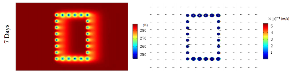
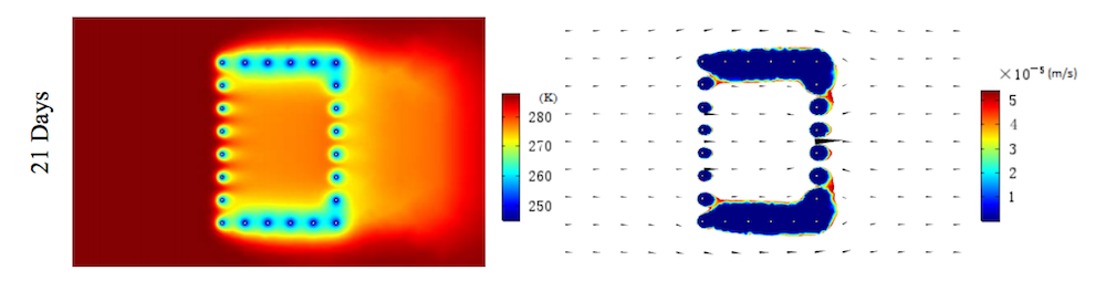
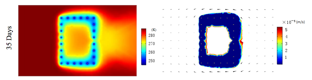
The temperature distribution (left) and permeability coefficient results (right) at various points in time. Images by Rui Hu and Quan Liu and taken from their COMSOL Conference 2016 Munich paper.
When comparing the closure of the freezing wall and flow velocity, the closing time increases nonlinearly as the flow velocity increases. The time of closure dramatically increases when the velocity is greater than 1.5 m/d. As for the average wall thickness in all directions and relative flow velocity, the influence of the flow velocity on the thickness of the upstream wall is most prominent.
The successful validation of this model offers guidance for the metro tunnel project in Guangzhou, China. With plans to further develop this model, the researchers hope to use it as a resource for improving applications of the AGF method.
Learn More About Modeling Subsurface Flow with COMSOL Multiphysics®
- Read the full COMSOL Conference paper: “Simulation of Heat Transfer during Artificial Ground Freezing Combined with Groundwater Flow“
- Browse some additional examples of modeling subsurface flow:

Comments (1)
Cahya
August 29, 2023Dear Bridget Cunningham,
I am very interested in your work on artificial ground freezing (AGF). Can you help me send this model file? I am currently studying AGF in college. Thank You
Best regards,
Cahya