
Many of our users are well aware of the fact that COMSOL Multiphysics can be used to solve partial differential equations (PDEs) as well as ordinary differential equations (ODEs) and initial value problems. It may be less obvious that you can also solve algebraic and even transcendental equations, or in other words, find roots of nonlinear equations in one or more variables with no derivatives in them. Are there real applications for this? Absolutely!
A Non-Ideal Gas Law
Consider a case where you are running a CFD simulation resulting in a velocity field, u=(u,v,w), and a pressure field, p. Now, let’s say that at the same time you wish to solve for convection and conduction of a temperature field, T, in a gas:
In addition, let’s assume that the density, \rho, is given by the ideal gas law:
To solve this you can simply substitute the expression for \rho as a function of T in the heat equation. This will result in:
where all quantities are known except for T, which you now solve for with COMSOL.
This is easy; the ideal gas law is a state law that allows us to access \rho(T) in a closed algebraic form suitable for direct substitution.
However, let’s now consider a case where the ideal gas law won’t do. This could be, for example, if you have a gas of high molecular weight at high pressures. Schematically, such a state law could look like this:
If you are interested in the physical parameters of such a state law, check out this resource.
This is a third-degree equation in \rho and we would like to solve for \rho. You can do this in principle, but it is quite cumbersome and we must not forget that the equation will in general have three roots. You can read on how to solve such equations by hand in this resource on cubic functions.
There is something about this task that one may not immediately realize: since p is a (assumed known) pressure field in space, we actually have one third-degree polynomial equation to solve for at each point in space within our CFD domain. We could call this an algebraic field equation or a distributed algebraic equation. Solving for all those roots manually is not a very manageable task. Instead we would need to rely on the solvers in COMSOL to do it. How are we to proceed?
We can conceptually view this algebraic equation as a degenerate form of a partial differential equation with neither space nor time derivatives. There are several ways of formulating such an equation in the COMSOL environment. For example, by using the Coefficient Form PDE interface or the Domain ODEs and DAEs interface. Using the Coefficient Form PDE interface, we would just zero-out all the coefficients of the space- and time-derivative terms and solve using a Stationary Study. Using the Domain ODEs and DAEs interface is perhaps a bit easier since there are no space-derivative terms to begin with.
Using the Domain ODEs and DAEs Interface
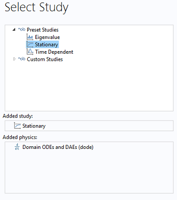
Let’s now have a look at a quick example based on the aforementioned non-ideal gas law. We want to start by selecting the Domain ODEs and DAEs interface in the Model Wizard:

To solve an algebraic equation, we should use a Study that is Stationary. This is done in the next step in the Model Wizard and will utilize the default damped Newton solver, which is general enough for most root solving purposes:
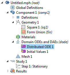
After finishing the Model Wizard, this is how the model tree will appear:
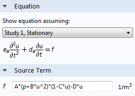
By default, the equation settings window for the Distributed ODE looks like this:
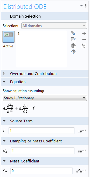
The unknown field variable representing the density is here called u (but we could easily change this to rho if we wanted to). We may now set the d_a coefficient to zero. However, since we already chose a Stationary Study, the time-derivative terms of this equation will not be considered by the solver, so we could also choose to leave it as is. In this case, the only thing that matters is what we put in the Source Term. Next, we type the equation for the non-ideal gas law into the source term, using the variable name u for the density:
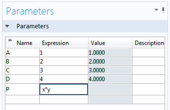
All that remains is to define the coefficients A, B, C, and D, as well as the given pressure field p. We will now do a few simplifying assumptions.
Let’s assume that our CFD domain is a simple unit square in 2D. In addition, we assume here that the pressure field is spatially varying as p(x,y)=xy and we will choose to work with dimensionless units. In a real case, this pressure field would of course be taken from the results of a CFD simulation solved together with this equation. We will also assign some arbitrary numbers to these coefficients: A=1, B=2, C=3, and D=4. This can all be done by defining Parameters under Global Definitions as follows:
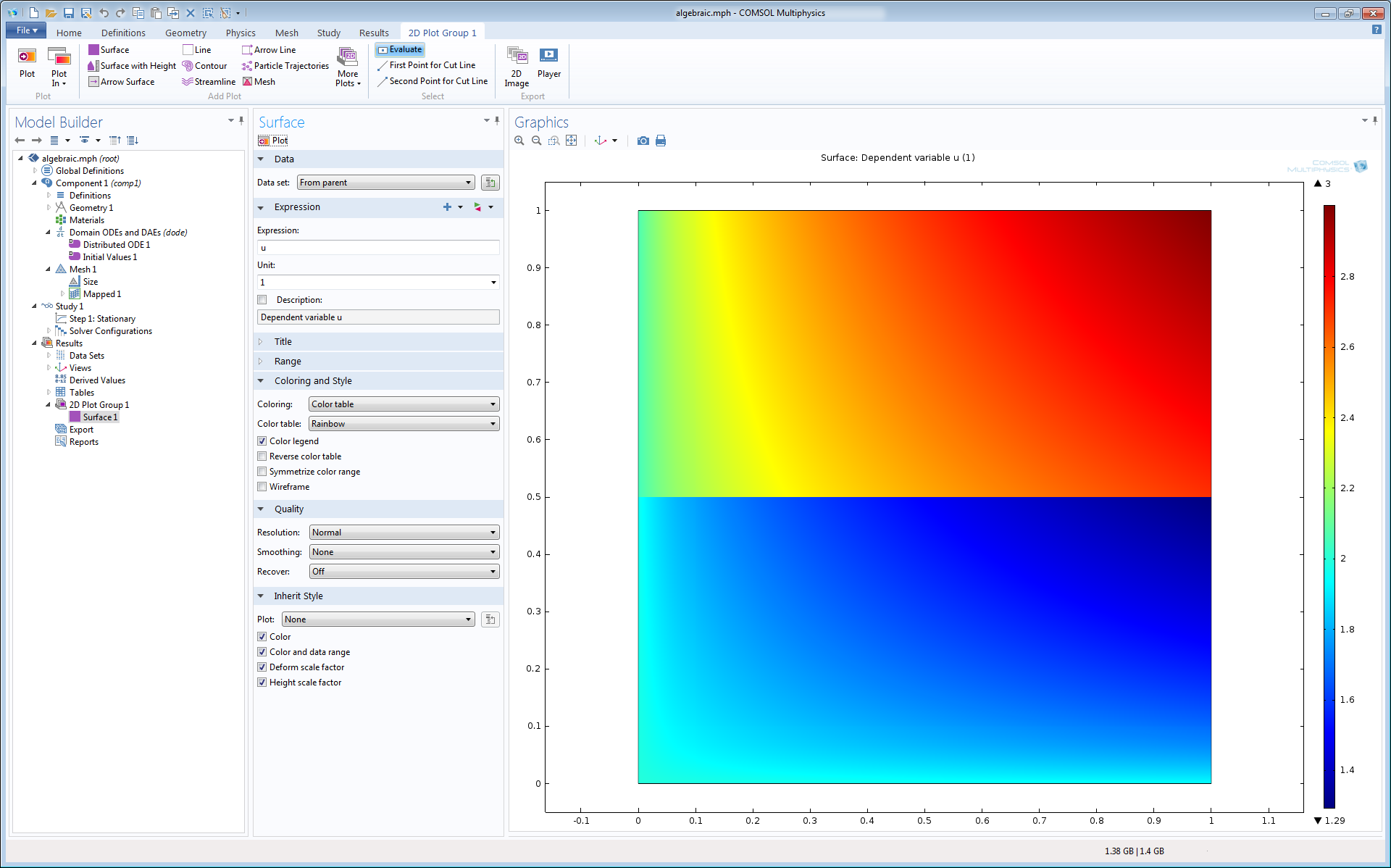
After doing so, we can solve this equation and get the resulting density field:
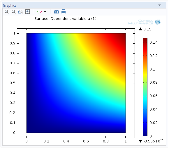
This surface plot shows the solution to the third-degree polynomial equation for each value of p throughout the unit rectangle.
Handling of Multiple Roots
For each value of p, at each point, the above plot shows only one of three possible solutions corresponding to the three roots of the equation. There may be additional continuity criteria that we would need to impose on the solution based on physical considerations. For example, if some of the roots are complex-valued, we may be able to ignore them. We could have a case where the solution abruptly changes from one physically realizable root to another in the middle of the domain. Such an event would perhaps correspond to a phase transition, such as going from a liquid to a gas.
How do we know which of these solutions we get? In general, this is a hard question to answer. If we are running a transient simulation alongside an algebraic state law, then the time-history may determine which root branch that the state law will slide into — at each point in space. When using a stationary solver, the root that is found may be determined by the Initial Value settings that are then used by the Newton solver as a starting point for its iterations, and then on the convergence region of the solver with respect to that starting point. Furthermore, the choice of discretization scheme, such as which element order and which type of finite element, may impact which roots are chosen by the solver.
To see what can happen, let’s experiment with an easier equation:
If we solve this by hand we get:
so that if we solve this on our unit square, we would get a unique solution u=2 at (0,0) and u=1 or u=3 at (1,1). If we now enter this simpler equation in COMSOL using the same methods as outlined above, we will get the following results for two different Initial Values:
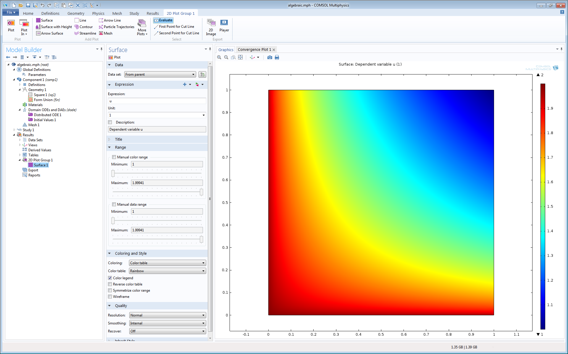
The solution with uniform initial value 1.9.

The solution with uniform initial value 2.1.
Note that in the general case, we may use an inhomogeneous distribution of initial values and get different roots in different parts of the computational domain:
The solution with a non-uniform distribution of initial values: u=1.9*(y=0.5). Here, the mesh is aligned with
the step defined by this initial value distribution and inter-element smoothing is turned off.
Conclusion
For certain types of simulations, it may not be enough to solve just the governing partial differential equations. COMSOL Multiphysics has the capability to solve for algebraic equations alongside the conventional physics interfaces, such as those for fluid flow, which may be critical for more advanced physics simulations. The capabilities don’t stop at algebraic equations, but could also include so-called transcendental equations, including functions such as sin() or cos() or even more general equations involving integrals. The examples above all use the core functionality of COMSOL Multiphysics.

Comments (2)
Pavel Kliuiev
January 17, 20141) Can one use this approach for analytic definition of an electromagnetic field in Waveoptics module? As an alternative for launching fields via Port BC?
2) I have COMSOL 4.3b and having problems with defining constant p=x*y in parameters. x*y look just red. How can I tell COMSOL that these are the coordinates?
Thanks for your answer
Bjorn Sjodin
March 12, 2014Hi Pavel,
1) This would be possible but not necessary since such computations are built-in to the Wave Optics Module in the very powerful port type boundary conditions. For example, the Wave Optics Module functionality allows you to compute the field at a port using a mode analysis or by defining a known electromagnetic field shape using mathematical expressions.
2) Yes, the Parameters list doesn’t “understand” the units of x and y since p=x*y is defined globally and does not belong to a particular model component. The model could, in principle, contain a mixture of 1D, 2D, and 3D components where there could be any number of spatial variables defined. Instead, to get unit handling on an expression like p=x*y you can define it as a Variable under Component->Definitions. This way the x and y variables are bound to one particular component. (The Parameters list was used here as a very quick way of achieving the results.)
I hope this helps,
Bjorn