

When using the COMSOL Multiphysics software to simulate wave electromagnetics problems in the frequency domain, there are several options for modeling boundaries through which a propagating electromagnetic wave will pass without reflection. Here, we will look at the Lumped Port boundary condition available in the RF Module and the Port boundary condition, which is available in both the RF Module and the Wave Optics Module.
Simplify Your Modeling with Boundary Conditions
When modeling electromagnetic structures (e.g., antennas, waveguides, cavities, filters, and transmission lines), we can often limit our analysis to one small part of the entire system. Consider, for example, a coaxial splitter as shown here, which splits the signal from one coaxial cable (coax) equally into two. We know that the electromagnetic fields in the incoming and outgoing cables will have a certain form and that the energy is propagating in the direction normal to the cross section of the coax.
There are many other such cases where we know the form (but not the magnitude or phase) of the electromagnetic fields at some boundaries of our modeling domain. These situations call for the use of the Lumped Port and the Port boundary conditions. Let us look at what these boundary conditions mean and when they should be used.
The Lumped Port Boundary Condition
We can begin our discussion of the Lumped Port boundary condition by looking at the fields in a coaxial cable. A coaxial cable is a waveguide composed of an inner and outer conductor with a dielectric in between. Over its range of operating frequencies, a coax operates in Tranverse Electro-Magnetic (TEM) mode, meaning that the electric and the magnetic field vectors have no component in the direction of wave propagation along the cable. That is, the electric and magnetic fields both lie entirely in the cross-sectional plane. Within COMSOL Multiphysics, we can compute these fields and the impedance of a coax, as illustrated here.
However, there also exists an analytic solution for this problem. This solution shows that the electric field drops off proportional to 1/r between the inner and outer conductor. So, since we know the shape of the electric field at the cross section of a coax, we can apply this as a boundary condition using the Lumped Port, Coaxial boundary condition. The excitation options for this condition are that the excitation can be specified in terms of a cable impedance along with an applied voltage and phase, in terms of the applied current, or as a connection to an externally defined circuit. Regardless of these three options, the electric field will always vary as 1/r times a complex-valued number that represents the sum of the (user-specified) incoming and the (unknown) outgoing wave.
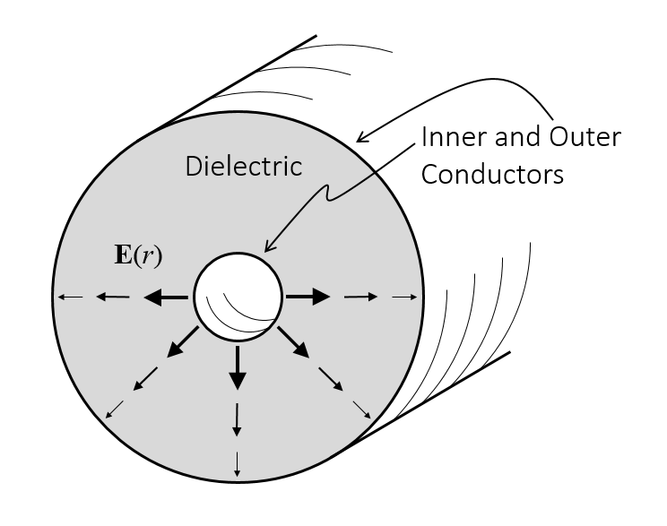
The electric field in a coaxial cable.
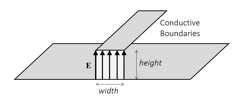
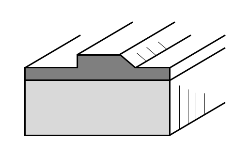
For a coaxial cable, we always need to apply the boundary condition at an annular face, but we can also use the Lumped Port boundary condition in other cases. There are also a Uniform and a User-Defined option for the Lumped Port condition. The Uniform option can be used if you have a geometry as shown below: a surface bridging the gap between two electrically conductive faces. The electric field is assumed to be uniform in magnitude between the bounding faces, and the software automatically computes the height and width of the Lumped Port face, which should always be much smaller than the wavelength in the surrounding material. Uniform Lumped Ports are commonly used to excite striplines and coplanar waveguides, as discussed in detail here.
A typical Uniform Lumped Port geometry.
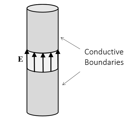
The User-Defined option allows you to manually enter the height and width of the feed, as well as the direction of the electric field vector. This option is appropriate if you need to manually enter these settings, like in the geometry shown below and as demonstrated in this example of a dipole antenna.
An example of a User-Defined Lumped Port geometry.
Another use of the Lumped Port condition is to model a small electrical element such as a resistor, capacitor, or inductor bonded onto a microwave circuit. The Lumped Port can be used to specify an effective impedance between two conductive boundaries within the modeling domain. There is an additional Lumped Element boundary condition that is identical in formulation to the Lumped Port, but has a customized user interface and different postprocessing options. The example of a Wilkinson power divider demonstrates this functionality.
Once the solution of a model using Lumped Ports is computed, COMSOL Multiphysics will also automatically postprocess the S-parameters, as well as the impedance at each Lumped Port in the model. The impedance can be computed for TEM mode waveguides only. It is also possible to compute an approximate impedance for a structure that is very nearly TEM, as shown here. But once there is a significant electric or magnetic field in the direction of propagation, then we can no longer use the Lumped Port condition. Instead, we must use the Port boundary condition.
The Port Boundary Condition
To begin discussing the Port boundary condition, let’s examine the fields within a rectangular waveguide. Again, there are analytic solutions for propagating fields in waveguide. These solutions are classified as either Transverse Electric (TE) or Transverse Magnetic (TM), meaning there is no electric or magnetic field in the direction of propagation, respectively.
Let’s examine a waveguide with TE modes only, which can be modeled in the 2D plane. The geometry we will consider is of two straight sections of different cross-sectional area. At the operating frequency, the wider section supports both TE10 and TE20 modes, while the narrower supports only the TE10 mode. The waveguide is excited with a TE10 mode on the wider section. As the wave propagates down the waveguide and hits the junction, part of the wave will be reflected back towards the source as a TE10 mode, part will continue along into the narrower section again as a TE10 mode, and part will be converted to a TE20 mode, and then propagate back towards the source boundary. We want to properly model this and compute the split into these various modes.
The Port boundary conditions are formulated slightly differently from the Lumped Port boundary conditions in that you can add multiple types of ports to the same boundary. That is, the Port boundary conditions each contribute to (as opposed to the Lumped Ports, which override) other boundary conditions. The Port boundary conditions also specify the magnitude of the incoming wave in terms of the power in each mode.
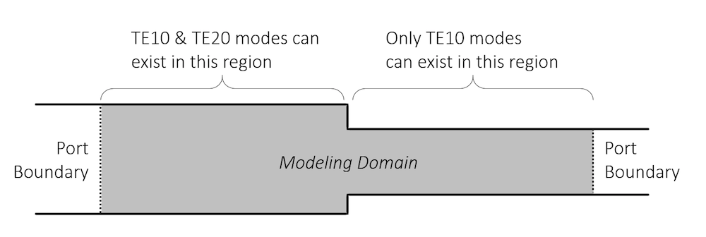
Sketch of the waveguide system being considered.
The image below shows the solution to the above model with three Port boundary conditions, along with the analytic solution for the TE10 and TE20 modes for the electric field shape. Computing the correct solution to this problem does require adding all three of these ports. After computing the solution, the software also makes the S-parameters available for postprocessing, which indicates the relative split and phase shift of the incoming to outgoing signals.
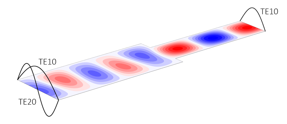
Solution showing the different port modes and the computed electric field.
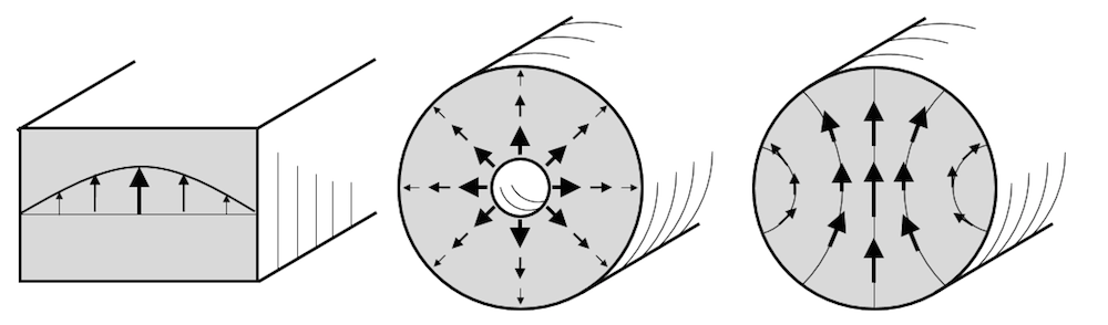
The Port boundary condition also supports Circular and Coaxial waveguide shapes, since these cases have analytic solutions. However, most waveguide cross sections do not. In such cases, the Numeric Port boundary condition must be used. This condition can be applied to an arbitrary waveguide cross section. When solving a model with a Numeric Port, it is also necessary to first solve for the fields at the boundary. For examples of this modeling technique, please see this example first, which compares against a semi-analytic case, followed by this example, which can only be solved by numerically computing the field shape at the ports.
Rectangular, Coaxial, and Circular Ports are predefined.
Numeric Ports can be used to define arbitrary waveguide cross sections.
The last case, when using the Port boundary condition, is appropriate for the modeling of plane waves incident upon quasi-infinite periodic structures such as diffraction gratings. In this case, we know that any incoming and outgoing waves must be plane waves. The outgoing plane waves will be going in many different directions (different diffraction orders) and we can determine ahead of time the directions, albeit not the relative magnitudes. In such instances, you can use the Periodic Port boundary condition, which allows you to specify the incoming plane wave polarization and direction. The software will then automatically compute all the directions of the various diffracted orders and how much power goes into each diffracted order.
For an extensive discussion of the Periodic Port boundary condition, please read this previous blog post on periodic structures. For a quick introduction to the use of these boundary conditions, please see this model of plasmonic wire grating.
Summary
We have introduced the Lumped Port and the Port boundary conditions for modeling boundaries at which an electromagnetic wave can pass without reflection and where we know something about the shape of the fields. Alternative options for the modeling of boundaries that are non-reflecting in cases where we do not know the shape of the fields can be found here.
The Lumped Port boundary condition is available solely in the RF Module, while the Port boundary condition is available in the Electromagnetic Waves interface in the RF Module and the Wave Optics Module as well as the Beam Envelopes formulation in the Wave Optics Module. This previous blog post provides an extensive description of the differences between these modules.
But what about those boundaries that are not transparent, such as the conductive walls of the waveguide we have looked at today? These boundaries will reflect almost all of the wave and require a different set of boundary conditions, which we will look at next.


Comments (8)
Mohand Alzuhiri
October 24, 2015dear is it possible to simulate a rectangular waveguide in time domain solver because there is no special waveguide port, i have tried it with lumped port with uniform geometry but the results doesnt look ok
Walter Frei
October 26, 2015Dear Mohand, Indeed, this series of articles is only discussing frequency-domain EM modeling, so time-domain is a bit outside of the scope. Briefly speaking: in the time domain, boundary conditions vary in space and time. The variation in time typically introduces some spread of frequency content into the signal, unless a Gaussian window is applied to any excitation pulse. To see a general example of how to apply such a Gaussian window, please see:
http://www.comsol.com/model/second-harmonic-generation-of-a-gaussian-beam-rf-956
Of course, if you’re trying to apply some different type of time-excitation, COMSOL gives you that flexibility as well.
Khoa Phan
August 20, 2016Hi,
in the case of output port in the tutorial Frequency Selective Surface, can anyone explain why the output port has Input quantity and why magnetic field is chosen as the input? It is supposed to be out put and COMSOL will calculate the field at it with the given input field at the input port, right?
Sevde Etoz
September 22, 2016Hello,
How can we calculate the reflected power at the lumped port ?
Thanks
Junlong Kou
January 25, 2017Hi, Walter,
I am quite confused when you say “Lumped Port and the Port boundary conditions for modeling boundaries at which an electromagnetic wave can pass without reflection”. But as far as I know, these ports can give quite accurate results on reflection. What do you mean by “without reflection”? Maybe I misunderstood something. Best,
Walter Frei
January 25, 2017Hi Junlong,
See, for example, the image of the 2D waveguide with a step-change in cross-section. A guided mode (TE10, 20) will pass through the port boundary condition without reflection. The port boundary condition thus mimics a moundary to an infinite (reflectionless) waveguide section.
Medani Sangroula
October 23, 2018Hi Walter,
I am a very new user to Comsol however, I used CST Microwave Studio to simulate S-parameters of different RF component previously. I am trying to simulate S_21 parameter for a simple coaxial structure (with respective diameters of the inner and outer conductor as 0.5 mm and 22 mm) that has a length of about 200 mm and is made out of copper. I put air-interface between the inner and outer conductor and would like to compare its S_21 parameter with CST. However, I could not assign a lumped coaxial port at its ends (the boundary did not get selected by somehow). I watch a couple of online videos but could not figure out.
Would you please let me know how can I fix this issue? Thank you.
Brianne Costa
October 29, 2018Hello Medani,
Thanks for your comment.
For questions related to your modeling, please contact our Support team.
Online Support Center: https://www.comsol.com/support
Email: support@comsol.com