

Today, we welcome a new guest blogger, Alexandre Oury of SIMTEC. He discusses the analysis of current distributions in a molten salt electro-refiner.
In a webinar highlighting electrochemical recycling processes, SIMTEC presented a computational approach for predicting current distributions in a molten salt electro-refiner. The three main types of current distribution (primary, secondary, and tertiary) were treated, with a particular emphasis on the first two types. Using COMSOL Multiphysics, we implemented primary and secondary current distributions in an electrolysis cell.
Molten Salt Electro-Refining
A common pyrometallurgical route for the recovery of many metals and rare earths is high-temperature molten salt electrolysis. This process involves a molten electrolyte made of a molten salt in which the metal to be recovered, most commonly present in its oxide form, is dissolved. When a current is applied between the cathode and anode, the metal is deposited as a solid or a liquid at the cathode, while some gas (generally a carbon oxide, such as CO or CO2) evolves at the carbon-based anode, as depicted in the figure below.
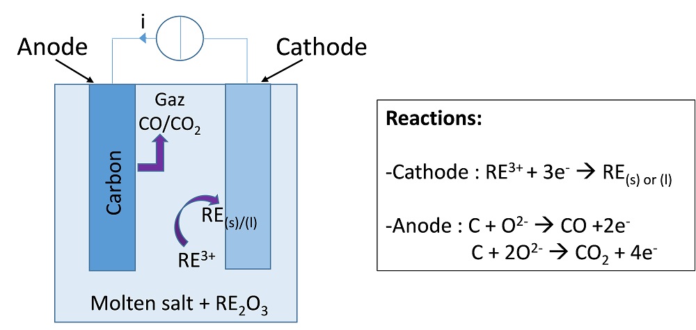
Principle of a molten salt electrolysis cell for the refining of rare earths.
Numerical simulation can be advantageously employed to predict the main cell features (e.g., the reaction rate distribution on the electrodes, the cell voltage, or the electrolyte temperature) in order to optimize the design and operational conditions of the process. Even though high-temperature electrolysis involves many physical phenomena that are complex and strongly coupled to one another, the reaction rate distribution on the electrodes can be approximated with a rather simple electrostatic approach that involves the calculation of the current densities associated with the reactions.
Simulating the Current Distribution
The current flow in an electrochemical device can be described by three different types of distributions: primary, secondary, and tertiary. The type of distribution depends on the reaction kinetics and whether the cell is limited by the transport of active species.
The primary current distribution assumes that the reaction kinetics are so fast that no reaction overpotential is associated with the activation of the reactions. The cell can be considered a simple resistive charge conductor. The only equation to solve is the conservation of the current density in all domains. An example of the equation and possible boundary conditions to implement in order to compute the primary current are represented schematically in the following image. In this example, the cathode potential is arbitrarily set to zero, while a current is prescribed at the anode.
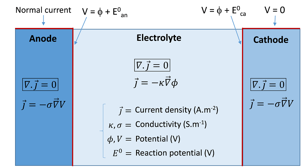
An example of equations and boundary conditions of a primary current model of an electrolysis cell.
The secondary current distribution accounts for the activation overpotentials of the reaction(s) at the electrode/electrolyte interfaces, which can be required when the electrochemical reactions are significantly slow. A kinetic relation is implemented as a boundary condition, which relates the electrode overpotential to the Faradaic current density. An ordinary kinetics expression is the so-called Butler-Volmer equation, which includes exponential activation terms. A schematic of the secondary current approach is illustrated below, with an example of a classical Butler-Volmer relation expressed with the exchange current density i0.
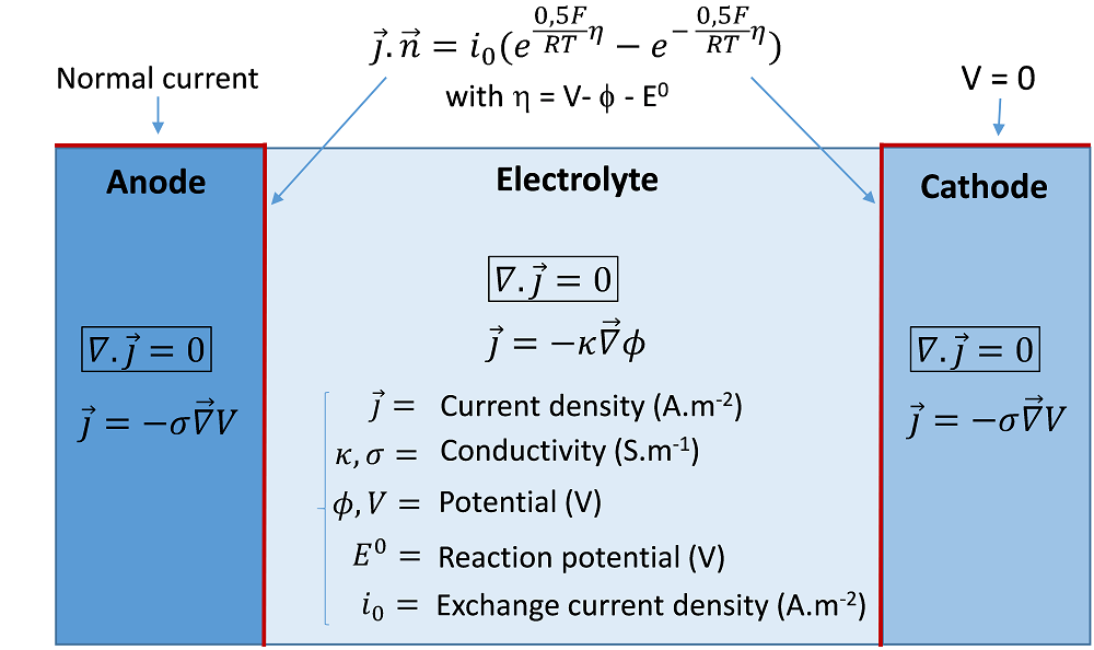
An example of equations and boundary conditions of a secondary current model of an electrolysis cell.
The design of the molten salt electro-refiner considered here is represented in the following figure. It is made up of several anode rods mounted in a circle around a central cathode rod. The electrodes are immersed in a molten salt-based electrolyte containing the metal (a rare earth, such as neodymium) to be recovered at the cathode. Symmetrical considerations allow the implementation of 1/32nd of the geometry without the loss of information, which significantly diminishes the degrees of freedom within the system.
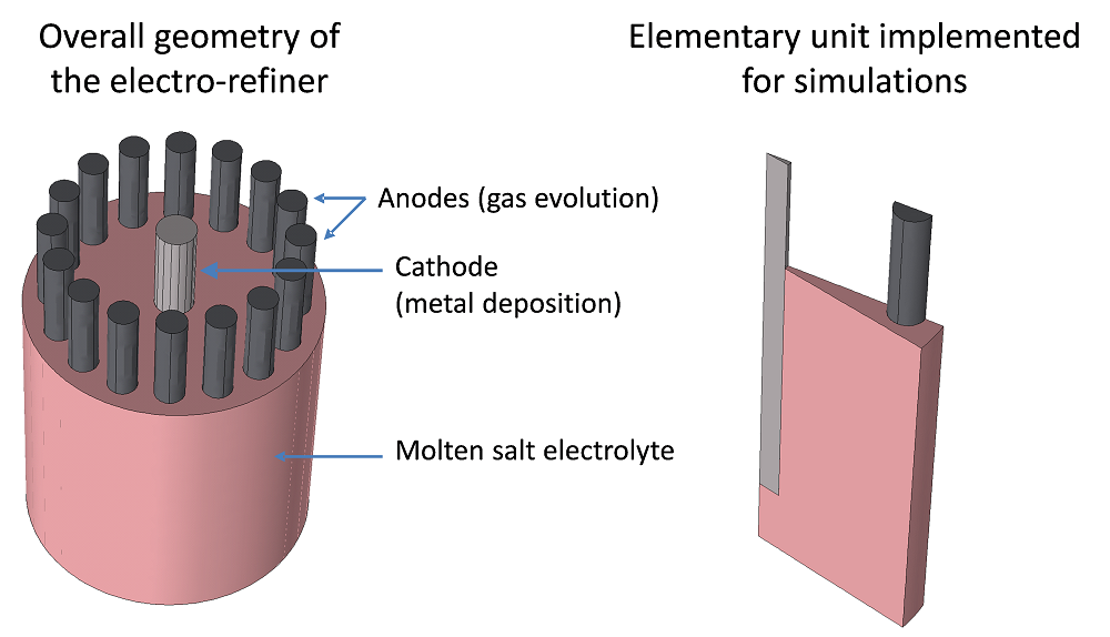
The geometry of the molten salt electro-refiner considered for simulation and an elementary unit obtained taking symmetry planes into consideration.
The primary and secondary current models are implemented in COMSOL Multiphysics using the Electric Currents physics interface of the AC/DC Module. Predefined physics interfaces are available in the electrochemistry-based COMSOL Multiphysics modules, such as the Electrodeposition Module, that provide easy definitions of terms such as the Butler-Volmer equations and enable the simulation of current distributions in electrochemical devices. However, we chose to use the Electric Currents physics interface found in the core COMSOL Multiphysics product and introduce the electrochemical reaction kinetics as expressions in the source term. Three electric currents physics are used, one for each domain (anode, cathode, and electrolyte). For both models, a Ground condition (V = 0) and a Normal Current Density condition are set on top of the cathode and on top of the anode, respectively.
In the case of the primary current model, the Electric Potential condition is set at both electrode surfaces, with the value defined in the primary current model example above. For the secondary current model, the Normal Current Density condition is used on these boundaries, selecting “Inward Current Density” with values defined by the Butler-Volmer relations in the previous secondary current model example. The conductivity of the electrodes and that of the electrolyte are set as constant. The kinetics parameters associated with the secondary current description are i0 = 1 A.cm-2 for the cathodic reaction and i0 = 0.001 A.cm-2 for the anodic reaction, corresponding respectively to fast (metal deposition) and slow (gas evolution) kinetics.
The domains are meshed using tetrahedral elements. There is no need for a special level of refinement. However, it is important to ensure that there are enough elements on top of the anode, where the current is injected, as well as on the electrode edges, where current peaks are expected (edge effects).
The current densities simulated at the electrode surfaces for a total prescribed current of 1000 Amps are shown for both models in the next image.
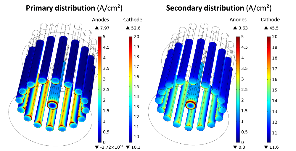
Current densities simulated at the electrode surface for the primary and secondary current models.
In both current approaches, it is observed that the gas evolution reactions on the anodes are mainly concentrated on the inner parts facing the cathode. The deposition rate is quite uniform along the cathode height, with a significant current peak taking place around the bottom edge. The main difference between the primary and secondary descriptions is the uniformity of the current associated with the anodic reaction.
In the case of a primary distribution, the current density ranges from 0 to nearly 8 A/cm². In the secondary distribution, the anodic current density range is twice as small, with a maximum value of 3.63 A/cm2. This is due to the homogenization effect induced by the activation overpotentials, which are accounted for in the secondary model. The difference between the primary and secondary currents is much more attenuated at the cathode, where a similar level of heterogeneity is observed due to the high value of i0 considered in the secondary model for the cathodic reaction.
The simulated cell voltages can be decomposed into several contributions. In the primary current model, the cell voltage (8 V) is the sum of the thermodynamic voltage \DeltaE0 (1.7 V) and the Ohmic drops occurring across the cell (6.3 V). In the secondary model, there is an additional activation term of 2.1 V due to the electrode kinetics, which brings the cell voltage up to 10 V.
The secondary current model is then expected to be more accurate than the primary model in terms of current and voltage, especially for such processes involving kinetically slow gas evolution reactions at the anode.
To bring the current model further, a tertiary distribution can be implemented to take into account the effect of the active species concentration in the electrode vicinity. However, such a model is more complicated as it requires an appropriate description of the species transport as well as the electrolyte convective motions in the cell. While an electrochemistry-based module, such as the Electrodeposition Module, has specific physics interfaces for defining and simulating tertiary current distributions, other physics sometimes need to be considered within the simulation. In our case, gas evolution at the anode as well as natural convection occurring through thermal gradients can affect the electrolyte concentration near the anode.
An example of bubbly flow simulated in the multi-anode cell with the Laminar Bubbly Flow interface is given in the following figure. It is shown that the main electrolyte movement occurs around the anodes where gas bubbles are released and rise, while slower zones are also apparent, for example, at the bottom of the cathode.
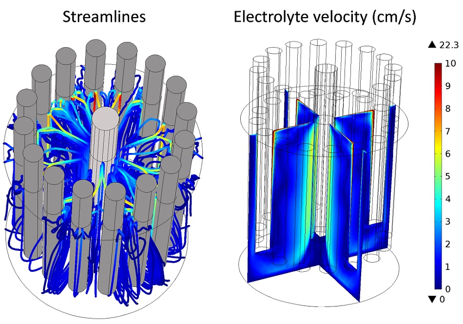
An example of a bubbly flow simulation in the electro-refiner.
Conclusion
In this short presentation, we reported on two current models developed with COMSOL Multiphysics for simulating the electrochemical reaction rate distribution in a typical molten salt electrolysis cell. The primary current model considers the reactions to be infinitely fast, while the secondary current model includes kinetics relations at the electrode/electrolyte interface. The results differ in terms of current uniformity (more uniform distributions for the secondary distribution) as well as cell voltage (significant contribution of the activation overpotentials in the secondary model). For such cells, a secondary approach is clearly better. While a tertiary current distribution is not presented, an example of the convective flow due to gas bubble formation at the anode is provided and can be used to solve for the tertiary currents.
About the Guest Author
Alexandre Oury received a master’s degree in materials science and engineering from Joseph Fourier University (Grenoble). He later earned his PhD in electrochemistry and process engineering from the National Polytechnic Institute of Grenoble, with a research topic related to battery storage systems. He currently works at SIMTEC as a modeling engineer, developing numerical models that are mostly applied to electrochemical systems and electrolysis cells.


Comments (7)
Larry Mickelson
November 2, 2017Dear Alexandre Oury,
Immediately after reading this blog post I attempted to construct simple models with primary and secondary current distributions using only the electric currents interface. I was able to develop a model with a primary current distribution. But I have been unable to construct a model of a secondary current distribution. I understand that I need to create a boundary condition with a current density source equal to the Butler Volmer equation. However, I can’t figure out how to define the overpotential needed to evaluate the Butler Volmer equation.
Could you provide further guidance?
Thanks,
Larry Mickelson, PhD
Staff Electrochemist
Alcoa
Patrick Namy
November 2, 2017Hi Larry,
thanks for your interest in our work!
You are right about the creation of a boundary between the 2 domains. Let’s imagine that the electric potential is denoted by V1 in the first domain, resp. V2 in the second one.
Your BV boundary conditions reads:
For V1, electric Currents 1, you will specify the inward current density by jC for instance
For V2, electric Currents 2, you will specify the inward current density by -jC (thus, conservation of the current)
and jC should be equal, for instance, to i0C*(exp(0.5*F_const*(V2-V1)/(R_const*T))-exp(-0.5*F_const*(V2-V1)/(R_const*T))).
Is it more clear like that? Do not hesitate to send me an email: patrick.namy@simtecsolution.fr
Larry Mickelson
November 17, 2017Hi Patrick,
Thank you for your help Patrick! The answer seems obvious now, but I simply couldn’t figure it out on my own. I had been trying to define a new variable, eta, but couldn’t figure out how to do so. However, I don’t need a new variable, all I need is V2 and V1! Much simpler, I applied this method to my model and was able to get it to work.
Thanks,
Larry Mickelson
P.S. Please forgive my slow response, I hadn’t expected anyone to answer so quickly and forgot to check back in.
Patrick Namy
November 21, 2017Fantastic Larry! I’m glad that my explanation makes things appear clearer now!
I hope you won’t hesitate to contact me directly by email if you need more information!
BTW, your solution (defining a new variable eta=V2-V1) could work too!!
Best,
Patrick
Nitish Gadgil
July 23, 2018Dear Alexandre Oury,
Thank you for documenting your work. It was quite clear to follow your approach. I have also gone through your article. The reason is, I am trying to simulate a gas evolving electrode- a planar 2D flat electrode. This means my gas evolution, unlike the domain gas evolution in your model, it would be through a boundary. Let me post my question first and then explain my model briefly: I run into negative gas volume fractions, no matter how fine my mesh size is. Did you face this issue during your model development?
More contrast from your model: I have a continuous electrolyte flow from bottom to top, through the cathode as well as the anode compartment. Simply put, imagine 2 compartments divided by a separator and the vertical boundaries of each compartment represent my electrodes.
I am using Tertiary current distribution with laminar bubbly flow. As mentioned above, I tried my model with several mesh sizes but gas keeps accumulating at the surface of anode and then leads to non-physical solutions. Assuming my boundary conditions are correct (which they are), it is hard to spot an obvious error.
Could you guide me a little further?
Thank you,
Kind regards,
Nitish Gadgil.
Master’s Student
TU Delft.
Patrick Namy
July 24, 2018Hi Nitish,
thanks for your post. I think your question would be more relevant to be submitted to the COMSOL support. Just a few tricks:
-) if you have negative concentration, perhaps it is due to high Pe Number. In that case, you need to monitor carefully your time step, maybe use artificial diffusion or express the concentration in a “log way”
-) perhaps your 2D geometry does not represent correctly the 3D one. It is often the case, when in 3D the gaz can leave the domain through one channel that is not described geometrically in 2D. Perhaps create “articificially” this channel to create an exit for the gaz?
Do not hesitate to contact me if needed,
kind regards,
Patrick Namy
Nitish Gadgil
July 24, 2018Dear Patrick,
Thank you for your extremely prompt response. I will try submitting the case to support. One more thing: would you clarify a little more about following lines from your response, I am still new to the software; terminologies are still sometimes puzzling.
-) What do you mean by expressing the concentration in “log way”? Is this for continuous and distributed phase both? Does Artificial diffusion correspond to Crosswind and streamline diffusion options in COMSOL?
-) I agree with you. I forgot to mention this in my question, but COMSOL creates this “artificial” channel extending in 3rd dimension.
Kind regards,
Nitish Gadgil