

If you’re looking for ways to manage multiple solutions, version 5.3 of the COMSOL Multiphysics® software offers several new tools for doing so. These include options for combining two solutions into one; storing solutions in different data sets so that they can be postprocessed and analyzed individually; and joining solutions to, for example, compare them. In this blog post, we will look at how to use these new tools.
Combining Solutions via Concatenation and Summation
Let’s say that we want to run a time-dependent simulation in two steps:
- From the starting time to an intermediate time
- From the intermediate time to an ending time
Further, let’s say that in the second time-dependent study step, we make some changes to the physics that represent a change in the conditions for the simulated device at the intermediate time. However, when postprocessing the results, we want to treat the output from the two study steps as a single continuous time-dependent solution.
We can achieve such a combined solution using the Combine Solutions study step, which is new in version 5.3 of COMSOL Multiphysics®. The Combine Solutions study step makes it possible to concatenate two solutions created in other study steps in the model. As an alternative to the concatenation of solutions (time-dependent or parametric solutions, for example), it is also possible to use summations to combine solutions (such as creating a solution that is the sum of various eigenmodes).
Example: Combining Two Time-Dependent Simulations
As an example of a concatenated solution, let’s look at the Axisymmetric Transient Heat Transfer example model. This model shows how a cylindrical object heats up when the temperature on its exterior boundaries changes from 0°C to 1000°C at the start of the simulation, which runs for 190 s.
Let’s see what happens if we add another time-dependent study step, which starts at 190 s where the boundaries are instead thermally insulated. To combine the two time-dependent simulations, a Combine Solutions study step provides a concatenation of the first and second study step. (In the settings, the second study step is called the Current solution, as it’s the solution computed in the step just above Combine Solutions.)
As a reference, we add a third time-dependent study step, which demonstrates that the heating of the boundaries continues uninterrupted during the time space of the two combined solutions. The study now contains the study steps shown below.
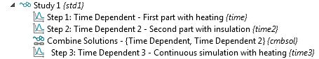
The study steps for a combined solution and a reference solution with only heating.
In the Settings window for the Combine Solutions study step, we specify the study steps to concatenate.
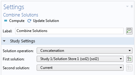
In the settings for the Combine Solutions study step, we can choose the type of solution operation and the solutions to combine.
When we compute the study, the study steps create corresponding solvers and Solution Store nodes in the solver configuration and also solution data sets for analyzing the results from the solvers. The data sets and corresponding solver configuration are shown below.
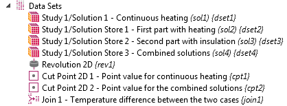
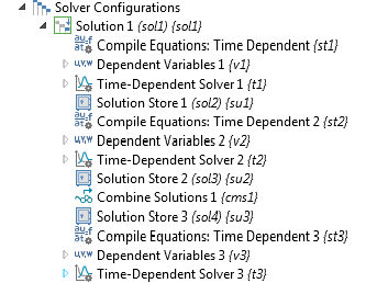
The data sets (left) and solver configuration (right). The top data set refers to the output from the third and final time-dependent study step.
In addition, we add the following data sets:
- A Revolution 2D data set to visualize the 2D axisymmetric solution in a corresponding 3D cylindrical geometry
- Two Cut Point 2D data sets to evaluate and plot a graph of the temperature in a reference location
- One of these data sets refers to the concatenated solution
- The other refers to the continuous solution
- A Join data set to evaluate and plot the difference between the concatenated solution and continuous solution
The following plot shows the temperature versus time for the concatenated solution, where heating is replaced by insulation after 190 s, and the continuous solution, where the heating continues during the time span of the entire simulation.
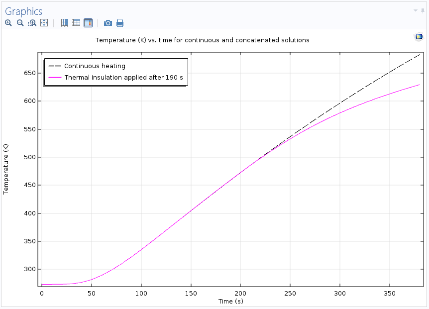
The concatenated solution (pink, solid) and the continuous solution (black, dashed). As expected, the temperature increase slows down when insulation is added.
Using a Join data set, we can plot the temperature difference between the two solutions. Until the point in time when insulation is added, the temperatures are the same, as expected.
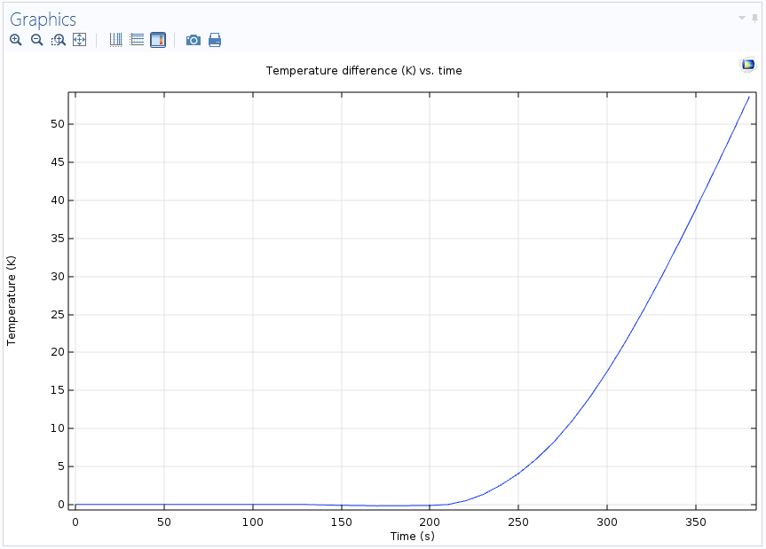
Temperature difference between the two solutions.
The temperature distribution in the full 3D geometry is available using the Revolve 2D data set.
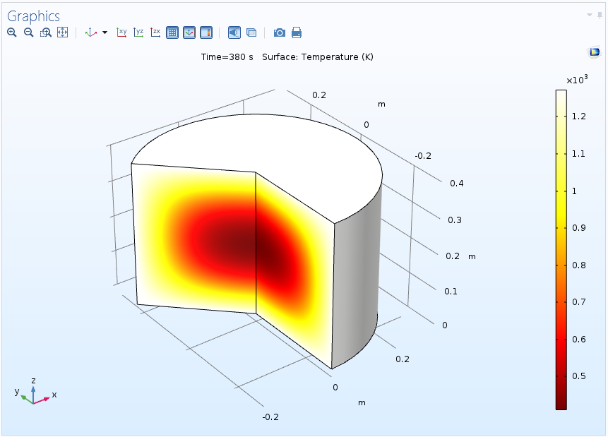
Temperature distribution in a segment of the full 3D geometry at the end of the continuous simulation.
Running a Simulation Multiple Times and Storing the Solutions in Different Data Sets
Another case where it is of interest to manage multiple solutions is when we run a simulation multiple times (with some variation in the model or settings) and want to postprocess and analyze the results from each run.
After computing an initial instance of the model, we right-click the Solver Configurations node in the study and choose Create Solution Copy to make a Solution – Copy solution and a corresponding data set available for our current solution (pointing to the Solution – Copy solution node under Solver Configurations).
When we then recompute with changes to the model or solver settings, the new solution is available through the original Solution data set, so that we can postprocess and evaluate both solutions by pointing to one of the two data sets (we can extend this approach to create additional solutions). We can also use a Join data set to combine solutions from two different Solution data sets (as a difference, for example).
Another option for creating additional Solution data sets is to right-click a Solution data set and choose Duplicate (or press Ctrl+Shift+D). The difference between this and the Solution Copy operation is that a duplicated Solution data set does not create a new solution and, by default, refers to the same solution as the original data set. For instance, we can use a duplicated data set to add a Selection node, if it is of interest to postprocess the solution in only a part of the model geometry. As of the latest version of COMSOL Multiphysics, Selection nodes are also available for most plot types in the plot groups. This enables us to directly hide boundaries for specific plots without having to create a separate data set, for example.
Example: Multiple Solutions for a Wrench Model
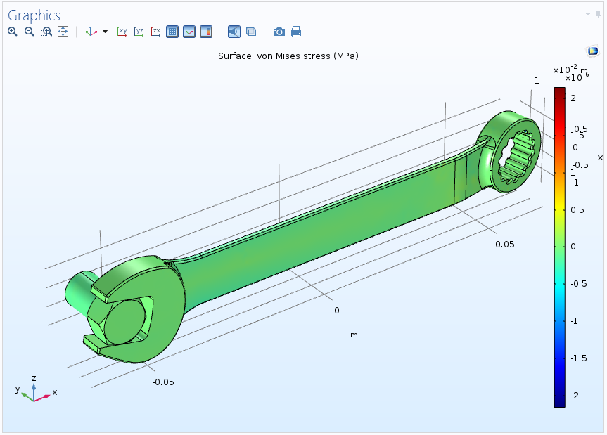
To illustrate these concepts, let’s open the Stresses and Strains in a Wrench example model.
One option is to use a parametric sweep or load case to investigate the stresses and deflections in the wrench for various forces applied as a boundary load at the end of the wrench. But let’s see what happens if the load’s direction is reversed so that the wrench is pulled upward (instead of pressed downward as it is in the example model from the Application Gallery). We can then store the original solution using a solution copy so that both cases can be postprocessed and analyzed individually.
To verify that the stresses are close to zero for a difference between the two cases, we also add a Join data set that contains the difference between the two solutions. By duplicating the original solution data set twice, we create two additional solution data sets — one for the wrench only and one for the bolt only — using Selection nodes. The model then contains the data sets shown below.
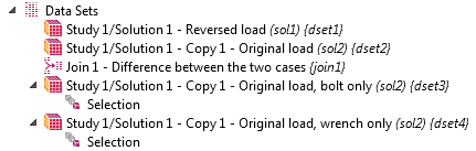
The wrench model’s data sets for comparing the two cases and for postprocessing using only the wrench and only the bolt.
The Solution data set on the left refers to the latest computed solutions; that is, the case where the load is reversed. The other Solution data set contains a copy of the first solution; that is, the cases with the original load direction.


The solution with a load acting upward (left) and the original solution, with a load acting downward (right).
The Join data set provides the difference between the two solutions above.
The difference in effective stresses is close to zero, evaluated using a Join data set.
The last two Solution data sets restrict the original solution to the bolt only and to the wrench only, defined by selections of boundaries that represent the bolt and the wrench, respectively.


Results for the wrench only (left) and the bolt only (right). These plots use data sets with applied selections.
It is now possible to analyze and plot the results in a flexible way for both load cases: for the difference between those solutions and for individual parts of the model’s geometry.
Concluding Thoughts on How to Manage Multiple Solutions in COMSOL Multiphysics®
These examples illustrate some of the flexible and powerful options that are available in version 5.3 of the COMSOL Multiphysics® software. The options for concatenating, using summations, and copying solutions make it possible to combine solutions for easier postprocessing as well as to store and analyze multiple solutions for different variants of a model. The options for duplicating and joining data sets make it possible to compare solutions and to visualize aspects of the same solution, perhaps for a certain part of the model. These tools are generally applicable and useful in many cases beyond what we have shown here.
Further Reading
- Learn more about Join data sets in this blog post: Solution Joining for Parametric, Eigenfrequency, and Time-Dependent Problems
- To get started with managing multiple solutions, download the tutorial models featured in this blog post:
- See other new features and functionality in COMSOL Multiphysics® version 5.3 on the Release Highlights page


Comments (24)
Antoni Artinov
June 22, 2017Dear Mr Ringh,
in COMSOL Multiphysics® wasn’t possible to use a transient multi solution as input under “Values of variables not solved for” by selecting “time: all” yet. The typical error was/is:
Selection “All” not available for multi solution
Error in multiphysics compilation.
An example for this is the automatically remeshed solution, which saves “one” solution on several meshes (multi solution).
…so is that possible now with the COMSOL Multiphysics® 5.3 version?
Best regards,
Antoni Artinov
Magnus Ringh
July 7, 2017Hi Antoni,
There are two types of “multi-solutions”:
* Multi-parametric solutions (for example, having “t” and other parameters as coming from Time-Parametric solutions).
* Solutions from time-adaption solutions, which are stored as several solutions for different meshes.
None of these can yet be handled with the “All” option for “Values of Variables Not Solved For” in Dependent Variables.
Best regards,
Magnus Ringh, COMSOL
Henry Ma
July 26, 2017Hi Mr. Singh,
I have been looking at the “Combine Solutions” feature to combine two separate study steps. I have noticed that if one of the studies has a different mesh than the first study, I come across the following warning:
“Reaction force in solution 2 is lost in concatenation”.
When plotting the results of the combined solutions, it looks like the mesh for solution 2 is lost, and all the results are with respect to the mesh for solution 1. Is this a feature intended?
Thank you,
Thanh Ma
Magnus Ringh
August 14, 2017Hi Tranh,
Yes, this is the intended behavior. Solution 2 is mapped to the mesh for solution 1. The concatenated solution will be for the mesh for solution 1.
Best regards,
Magnus Ringh, COMSOL
Alireza Rezaee
August 17, 2017is the model for the first example “Combining Two Time-Dependent Simulations” available online?
Magnus Ringh
August 18, 2017Hi Alireza,
The extension made in the blog example is not available online, but the model that it’s based on is available here, as noted in the blog: https://www.comsol.com/model/axisymmetric-transient-heat-transfer-267
Best regards,
Magnus Ringh, COMSOL
Alireza Rezaee
August 18, 2017Hi Magnus,
Thank you. I was wondering if it is possible to have access to the modified model (with extension)? I tried to go through the steps and I failed to get the model to run. is there any tutorial available for multiple steps and solution management?
Thanks
Alireza Rezaee
Magnus Ringh
August 18, 2017Hi Alireza,
If you have problems getting your model to run, I recommend that you contact the COMSOL support team. They will be able to help you with any questions regarding your model setup.
Best regards,
Magnus Ringh, COMSOL
Alireza Rezaee
August 20, 2017Magnus Ringh,
Thanks for your reply, I need a clarification on this topic.,
whats the difference between concatenation and summation? They don’t seem to be different and the documentation does not elaborate on it.
Thanks
Alireza Rezaee
Magnus Ringh
August 21, 2017Hi Alireza,
Concatenation is the most common (and the default) option: You can use it to join (concatenate) two time-dependent studies, for example, where one covers [t0, …, t1] and the other [t1, …, t2] so that you get one time-dependent solution for the entire time span [t0, …, t2]. Summation is the process of summing several solutions, such as multiple eigensolutions, to form a solution that is the sum of all “input solutions”.
Best regards,
Magnus Ringh, COMSOL
Hernán Felipe Garrido Pulgar
September 6, 2017Hi Magnus! How did you add the insulation study? Did you modify the “heat transfer” module that you had, or did you add another “heat transfer” module with the insultating property? I am very insterested! Thank you
Magnus Ringh
September 7, 2017Hi Hernán Felipe,
The model uses some powerful concepts in COMSOL Multiphysics. You only need to use one Heat Transfer in Solids interface, with a Thermal Insulation node added from the start, but followed by a Temperature node, which defines a fixed temperature on the same boundaries and thus “overrides” the thermal insulation. That is the setup for the first Time Dependent study step. In the second Time Dependent study step, which continues the simulation but with thermal insulation instead, the “Modify physics tree and variables for study step” check box is selected. You can then disable the Temperature node for that specific study step. By doing so, Thermal Insulation becomes the active boundary condition in the simulation part that the second Time Dependent study step controls.
Best regards,
Magnus Ringh, COMSOL
Bing Li
January 10, 2018is the model for the first example “Combining Two Time-Dependent Simulations” available online?
Magnus Ringh
January 10, 2018Hi Bing,
Yes, there is a link in the blog post that takes you to the Application Gallery, where the Axisymmetric Transient Heat Transfer example model is available:
https://www.comsol.com/model/axisymmetric-transient-heat-transfer-267
At least in the 5.3a version of that example model, a Combine Solution node is used to combine two time-dependent simulations into one (it is done under Study 2 in that model’s setup).
Jesus Lucio
January 14, 2018Hi Magnus,
Thanks for this helpful blog.
I have three small related questions:
1. What if we have more than 2 time steps? Cannot we combine all the solutions in one? It would be perfect if “Combined Solutions” could accept ANY number of (time) steps.
2. And what about ‘for’ loops? If we use a for loop, how can we have the solutions of all iterations saved, not just the last one?
3. And talking of ‘for’ loops, is there an iterator (an accessible variable, say ‘iter’ or whatever, taking the value of the iteration: 1, 2, etc.) that we can use, for instance in the time steps (like iter*t)?
Thanks in advance and regards,
Jesus.
Anonymous
January 15, 2018Hi Jesus,
Thanks! Great that you found this blog post to be helpful.
Please see below for answers to your three questions:
1. You can concatenate more than two solutions by using multiple Combine Solutions nodes and using the output from an earlier Combine Solutions node as one of the inputs to the following Combine Solutions node, in addition to another time-dependent solution that you want to concatenate to the previously concatenated solutions. Allowing more than two time steps in a single Combined Solutions node is an extension that we will consider.
2. The for-loops are designed to iterate between our main solvers (time-dependent, stationary, eigenvalue, and so on) to produce a solution (if the process converges). Inside such a loop you can have any solver feature (node). One such node can be a Solution Store or Copy Solution node. Those nodes will make a copy of the solution at each iteration of the loop and overwrite the solution stored from the previous iteration. There is currently no functionality (in the COMSOL Desktop) to add a new solution for each iteration. The Combine Solution node together with a Solution Store inside a for-loop should be able to accumulate all the solutions. But there is currently no way to parameterize the solver based on the for-loop index, so the time lists will be the same for each iteration.
3. Not yet, but it has been suggested before to introduce such a variable.
Best regards,
Magnus Ringh, COMSOL
Ralph Youngs
April 24, 2018what is causing solution number out of range when study is re-run with parameter change?
Magnus Ringh
April 25, 2018Hi Ralph,
It’s likely that some expression in some results plot or evaluation explicitly references a parameter value that is no longer part of the set of parameter values when you rerun the study.
Best regards,
Magnus Ringh, COMSOL
David Benson
October 9, 2018Hi
I have a question about solutions in COMSOL.
I am working on the energy pile performance (the energy pile, also called heat exchanger pile, is a pile equipped with individual or several pipe circuits in order to enable exchange of heat with the surrounding soil).
My main question is that how can i see the effect of pile’s temperature (which changes sinusoidally, see Fig. 1) and ground interior temperature (which varies from day to day, see Fig. 2) at the same time on every point? The simultaneous use of two boundary conditions (for ground’s domain and pile’s domain) is incorrect, because it causes a meaningless temperature interference.
For this reason, I wanted to produce the ground interior temperature using an mathematical expression in initial values node (and not in temperature node). This mathematical expression contains the variables z and t. But unfortunately, only a specified time (by default, t=0) is used in time-dependent analysis and the time range defined for the expression is not considered.
Now I do not know exactly what to do to solve this problem.
Fig. 1: https://www.comsol.com/forum/thread/attachment/407691/fig-1-4129a8d.jpg
Fig. 2: https://www.comsol.com/forum/thread/attachment/407691/fig-2-fbd42f4.jpg
Best regards,
David
Brianne Costa
October 10, 2018Hello David,
Thanks for your comment.
For questions related to your modeling, please contact our Support team.
Online Support Center: https://www.comsol.com/support
Email: support@comsol.com
K Vinay Kumar
January 6, 2019Dear Sir/Madam,
I have a query regarding on COMSOL Simulation
I’m doing Solar PV Cell with different structures by using a 2D model physics & I used electromagnetic waves and frequency domain, study I have used frequency domain, as result of that I get reflectance data for different wavelengths and after I tried to design the si_solar_cell_1D model as per the COMSOL design instruction procedure after simulated, I get the I-V and P-V Curve of solar cell.
but I will combine both frequency domain and semiconductor models in one simulation how to combine these two data by adding reflectance data in the in the generation and recombination of Solar PV cell 1D Model. In the si_solar_cell_1D model, how to add the reflectance data to that model and how to simulate that model.
Brianne Costa
January 7, 2019Hello K Vinay,
Thank you for your comment.
For questions related to your modeling, please contact our Support team.
Online Support Center: https://www.comsol.com/support
Email: support@comsol.com
biao feng
March 25, 2019Do I need to rerun the compute for the combined study to be effective? when I just set the node, I didn’t see the combined results available.
Magnus Ringh
March 26, 2019Hi Biao,
Once you have set up a study with, say, two Time Dependent study steps and a Combine Solutions study step, then running the complete study will provide the combined results. Make sure that you use a dataset that corresponds to the combined solution during postprocessing.
Best regards,
Magnus Ringh, COMSOL