

You can generate and visualize randomized material data with specified statistical properties determined by a spectral density distribution by using the tools available under the Results node in the COMSOL Multiphysics® software. In this blog post, we show examples that are quite general and have potential uses in many application areas, including heat transfer, structural mechanics, subsurface flow, and more.
Synthesizing Randomized Inhomogeneous Material Data
We have already discussed how to generate random-looking geometric surfaces by using sum and if operators in combination with uniform and Gaussian random distribution functions. The idea is that by summing up a set of spatially varying waves with careful choices of amplitudes and phase angles, we can mimic the type of randomness frequently found in natural materials and many natural phenomena in general.
To generate synthetic material data in 2D, we can use the same double-sum expression that we used to create randomized CAD surface data in the previous blog post:
Note that this sum could also be used to generate random data for use in boundary conditions on surfaces in a 3D model.
For the 3D volume case, we will need triple sums:
The frequency-dependent amplitudes will take their values from a random distribution according to
and
for the 2D and 3D cases, respectively.
The functions g(k,l) and g(k,l,m) have a random Gaussian, or normal, distribution and h(k,l) and h(k,l,m) are frequency-dependent amplitude functions with values that taper off for higher frequencies in accordance with the spectral exponent β. The higher the value of the spectral exponent, the smoother the generated data will be. For a variety of reasons, many natural processes have this property, which is characterized by slower variations that are more dominant than fast.
The phase angles φ are sampled from a function u. The function has a uniform random distribution that is between -\frac{\pi}{2} and \frac{\pi}{2}:
φ(k,l) = u(k,l) and φ(k,l,m) = u(k,l,m)
The sums run over a set of discrete frequencies. More nonzero terms in a sum imply a larger number of higher-frequency contributions, resulting in data that contains finer details. The maximum frequencies in each direction are determined by the integers K, L, and M, respectively. These types of sums are closely linked to discrete inverse cosine transforms. They essentially correspond to an inverse cosine transform of the amplitude coefficients g(k,l) and g(k,l,m), with some additional manipulations of the phase angles. For details, see the previous blog post on how to generate random surfaces in COMSOL Multiphysics.
Expressions for Double and Triple Summation
In COMSOL Multiphysics, the following double-sum expression can be entered in various edit fields, such as 2D material properties or 3D boundary conditions:
0.01*sum(sum(if((k!=0)||(l!=0),((k^2+l^2)^(-b/2))*g1(k,l)*cos(2*pi*(k*s1+l*s2)+u1(k,l)),0),k,-N,N),l,-N,N)
We can use a similar expression for the triple sum, which can be used for 3D material data, loads, sources, and sinks:
0.01*sum(sum(sum(if((k!=0)||(l!=0)||(m!=0),((k^2+l^2+m^2)^(-b/2))*g1(k,l,m)*cos(2*pi*(k*x+l*y+m*z)+u1(k,l,m)),0),k,-N,N),l,-N,N),m,-N,N)
where we have set K = L = M = N.
For more details about the underlying theory and syntax used here, see the blog post mentioned above.
Working with models that contain triple sums is computationally quite expensive. It is more efficient to first generate the data and export it to file and then import it again as an interpolation function, perhaps in a separate model. This interpolation function can then be used in a variety of ways, as we will explain later. Alternatively, you can use external software to generate the data by means of inverse FFT.
Let’s now take a look at how to generate 3D material data.
Generating a Randomized Interpolation Table in COMSOL Multiphysics®
Creating a 3D volume matrix of random data is surprisingly easy. It amounts to creating a couple of random functions, some parameters, a Grid data set, and an Export node.
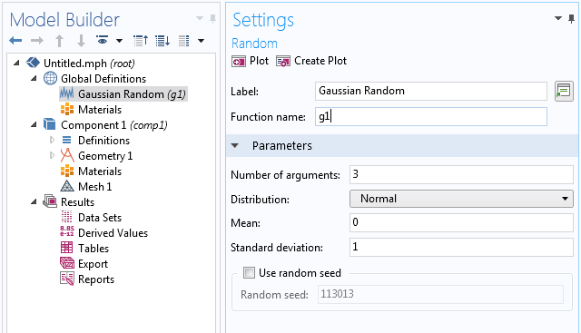
Start by creating a random function for the amplitudes with 3 input arguments based on a normal, or Gaussian, distribution. This corresponds to the function g(k,l,m) in the mathematical description above. In this case, we arbitrarily use the default settings for a random function with the mean value set to 0 and the standard deviation set to 1.
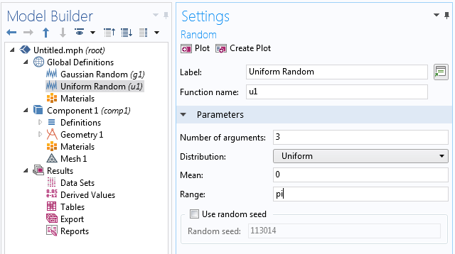
Next, we create a random function for the phase angles with 3 input arguments based on a uniform distribution between -\frac{\pi}{2} and \frac{\pi}{2} corresponding to the function u(k,l,m) above.
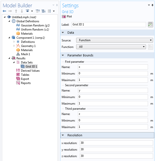
Now, create a data set of the type Grid 3D that references the random functions as a source. We need this data set to give an evaluation context to the triple-sum expression that we will define later in the Export node.
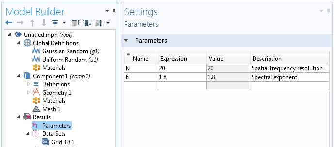
We will use two results parameters, N and b, for the spatial frequency resolution and spectral exponent, respectively.
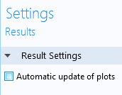
To make it easier to work with the large data sets that are generated, you can turn off the Automatic update of plots option. This setting is available in the Settings window of the Results node. Turning it off avoids recomputing the expressions each time you click on a plot group under Results.
To visualize the data before exporting to file, add a Slice plot and type (or paste) the expression:
0.01*sum(sum(sum(if((k!=0)||(l!=0)||(m!=0),((k^2+l^2+m^2)^(-b/2))*g1(k,l,m)*cos(2*pi*(k*x+l*y+m*z)+u1(k,l,m)),0),k,-N,N),l,-N,N),m,-N,N)

To export the data, add a Data node under Export and type in the same expression as for the Slice plot above. In the Settings window of the Data node, make sure to set the data set to Grid 3D and to specify a file name that the data will be written to. Here, we can let the points be evaluated in a way that is independent of the Grid 3D data set.
For the setting Points to evaluate in, select Regular grid. For Data format, select Grid. You can freely choose the number of x, y, and z points to evaluate in. In the figure below, these points have each been set to 50. Note that data generation corresponding to numbers higher than 50 may take a very long time to generate. For a 50x50x50 grid, we already get 125,000 data points.

The text file that is generated and exported can now be imported to a new file for the purpose of setting up a physics analysis where we use the generated data in material properties. This can be done for any type of physics, including electromagnetics, structural mechanics, acoustics, CFD, heat transfer, and chemical analysis. By using the COMSOL® API in methods or applications, for example, such export and import operations can be automated and set in the context of a for-loop in order to generate statistics over a larger sample set. In this example, we only generate one set of data.
Using the Generated Data in a Heat Transfer Analysis
To illustrate how this type of data can be used, let’s create a test model of the simplest possible kind, based on a heat transfer analysis.
Start by creating a new 3D model using a Heat Transfer in Solids interface.
Now, import the data from file as an Interpolation function. This function will be available under the Global Definitions node.
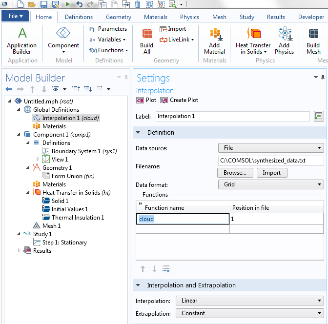
The Interpolation function is given the name cloud and can later be accessed using expressions like cloud(x,y,z).
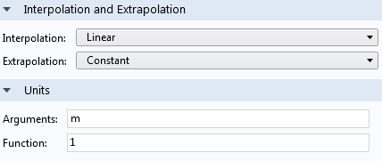
To make unit handling easy, when using this interpolation function, we will set the input argument units to m and the function unit to 1. The Function unit corresponds to the unit of f(x,y,z)=cloud(x,y,z) and setting it to 1 makes it dimensionless.
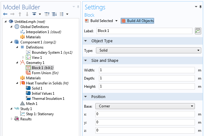
To keep things simple, let’s use a Block geometry object that matches the imported data exactly, with the corner at the origin and sides at 1. This corresponds to the size and position of the Grid 3D data set used earlier for generating the data.
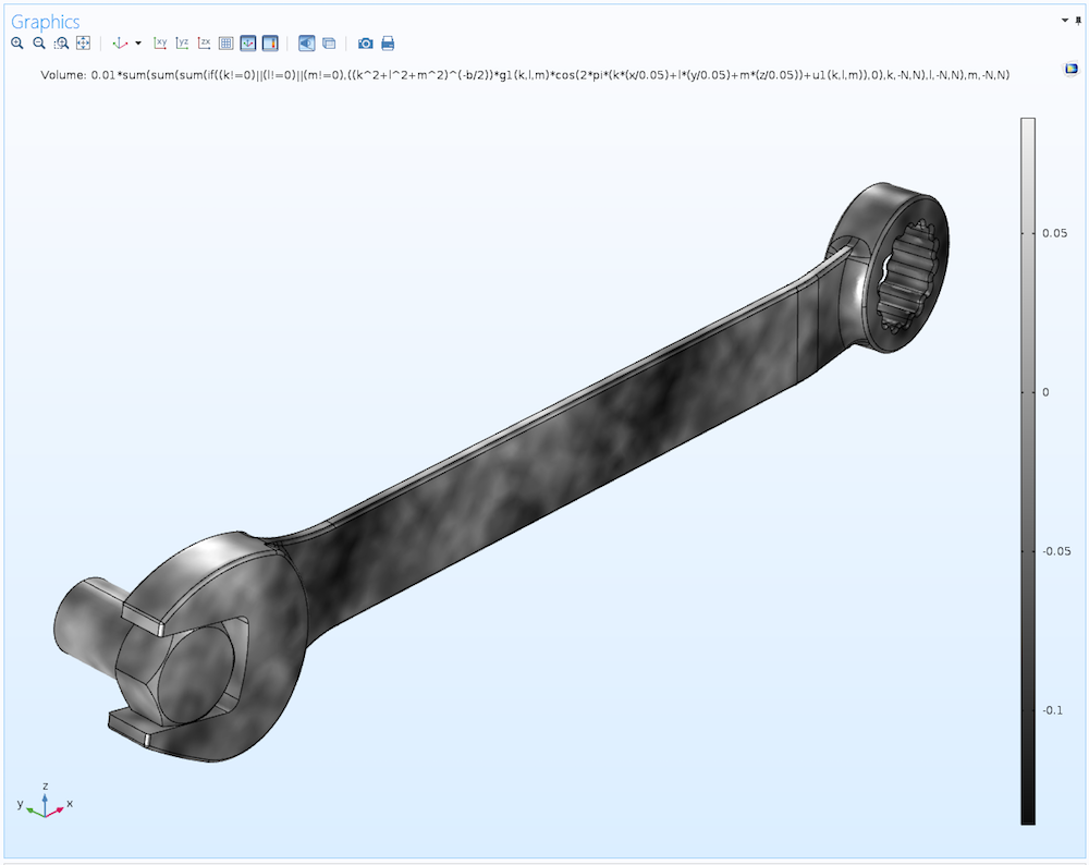
For a “real” case, you can instead import or create a CAD geometry, which can be used to truncate the interpolation function in a suitable way. This truncation of data is automatic in COMSOL Multiphysics. The figure below shows such an interpolation of randomized data over a CAD model of a wrench. When evaluating over an arbitrary geometry, it can be useful to scale the coordinate values in the triple-sum. In the wrench example, instead of k*x+l*y+m*z, as in the expressions above, the scaled expression k*(x/0.05)+l*(y/0.05)+m*(z/0.05) is used.
This type of irregular material data may have uses in statistical modeling of materials such as those found in additive manufacturing, where perfect material homogeneity of a 3D-printed component may not always be possible to achieve. The data can be used for any type of material property, such as conductivity, permeability, and elasticity properties, to name a few.
Getting back to our unit cube example, we now add a Blank Material node. We will, somewhat arbitrarily, set the Density to 2000 kg/m3 and the Heat capacity to 1 J/kg/K. Since we are performing a stationary analysis, the Heat capacity is irrelevant. The Thermal conductivity is set to the expression 1+2[W/m/K]*cloud(x,y,z). We can see from the earlier Slice plot visualization that the values for the interpolation table are roughly between -0.2 and 0.2. This means that this expression will generate an interesting spatial distribution of thermal conductivity values between about 0.6 and 1.4.
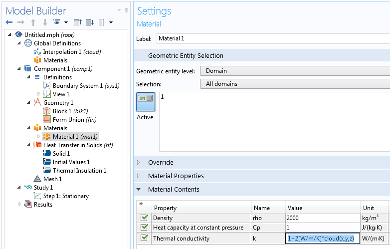
The coefficient 2[W/m/K] is used to assign a consistent unit to the expression. The constant 1 will be automatically converted to the correct unit: [W/m/K].
Let’s define some simple boundary conditions. Set the temperature at the top surface to 393.15[K] and the bottom surface to 293.15[K], corresponding to a 100-K temperature difference.

Now, let’s generate a default mesh.

COMSOL Multiphysics will automatically interpolate values such as those from the material properties to this unstructured mesh from the imported interpolation function. Alternatively, we could generate a swept mesh with hexahedral elements of the same size as the original data, 50x50x50. Such a representation would be more “true” to the original data.
You can experiment with different element orders, such as linear and quadratic types. Unless you use a very fine mesh that “oversamples” the data, the results will depend somewhat on the element order.
Running the Study will produce a couple of temperature plots, the second of which is an Isosurface plot.

Notice how the Isosurface plot looks a little bit jagged, which is due to the underlying irregularity of the material data. We can create another Slice plot to yet again visualize the data. This time, we do so under the guise of thermal conductivity by using the variable ht.kmean, which equals the expression 1+2[W/m/K]*cloud(x,y,z) defined earlier.

Here, the data is sampled at a lower sampling density than the original interpolation function, since we used the default mesh with the Element size set to the default Normal setting. Successively refining this unstructured mesh will ultimately sample the data at more or less the same level of detail as the original synthesized data.
As mentioned earlier, the approach used here for heat transfer is applicable to virtually any other type of simulation. For example, in a porous media flow simulation, the randomized quantity would be permeability rather than thermal conductivity. In the case of porous media flow, a more advanced random distribution may be needed, but let’s save that discussion for a future blog post.
Binary Data and Percolation Effects
We can also use the synthesized data in a different way: by using Boolean expressions to convert it to binary data. This method can be used for simulating two or more materials where the material interface is randomized and the material properties change abruptly from one point to another. COMSOL Multiphysics will automatically handle the sharp interpolations needed for this case.
The following picture shows a visualization of the Boolean expression cloud(x,y,z)>-0.03, which evaluates to 1 at points where the inequality is true and 0 at the other points.

To get a nicer plot, you can set the resolution of the Slice plot to Extra fine. This setting is available in the Quality section of the Settings window for the Slice plot.
We would now like to use this type of binary information in a simulation. It can be interesting, for example, to use it in a heat transfer simulation to see the so-called percolation effects. For certain threshold values, you get a large connected component in the material so that the entire slab of material starts conducting much more efficiently.
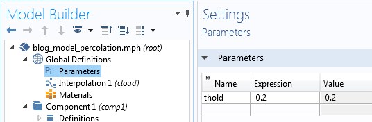
To try this, change the expression for the thermal conductivity to 1-0.9[W/m/K]*(cloud(x,y,z)>thold), where thold is a global parameter. Start by defining thold in Parameters under Global Definitions.
Then, change the material data accordingly.
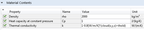
For each point in space, the Thermal conductivity will, in a binary fashion, evaluate to 1 or 0.1, depending on the value of the inequality.
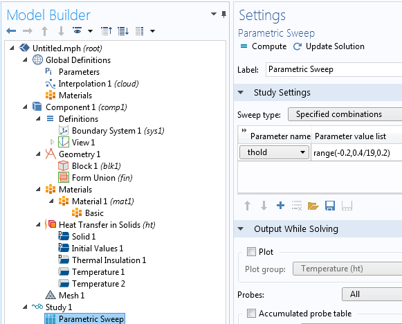
Now, let’s see how different values of this Boolean threshold will affect the simulation. For this purpose, run a parametric sweep over the parameter thold from -0.2 to 0.2.
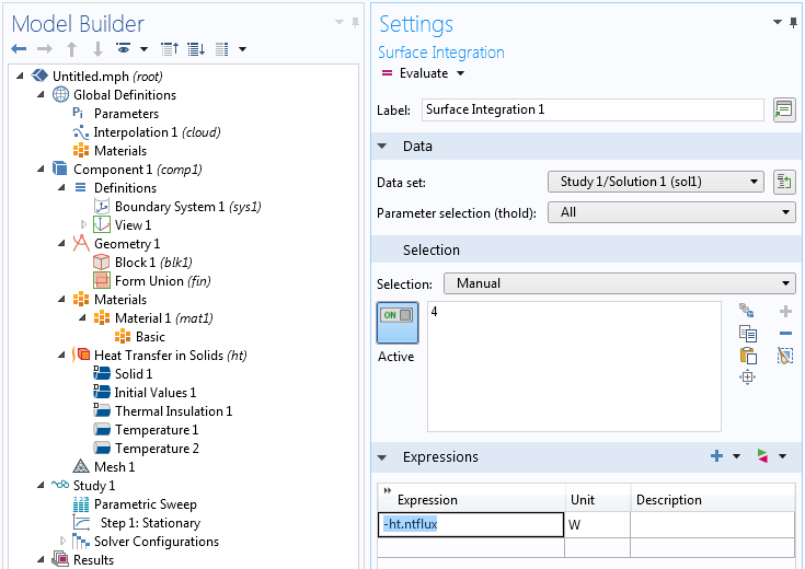
Add a Surface Integration node under Derived Values to integrate the total heat flux that goes through one of the surfaces. This will be given by the surface integral of -ht.ntflux or +ht.ntflux, depending on if you are integrating over the top or bottom surface. In the figure below, we used the top surface.
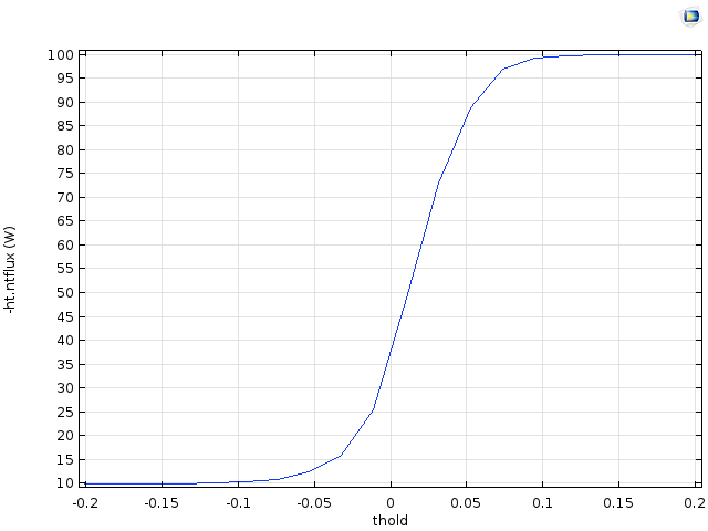
The resulting Table plot shows the amount of heat power transferred (in watts). We can see that for threshold values around 0, the conductivity rises quickly from a low value to a high value. This is due to the sudden appearance of one or more large connected components where the expression 1-0.9[W/m/K]*(cloud(x,y,z)>thold) evaluates to 1.
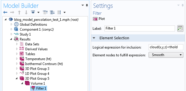
The figures below show a Volume plot with a Filter attribute for three threshold values around 0. The filter shows the parts of the domain for which cloud(x,y,z)<thold corresponds to the locations of higher conductivity.


We can see from these figures how the highly conductive parts start connecting for the higher threshold values.
The corresponding Filter settings are shown in the figure below.
A similar type of percolation effect, seen here for binary data, is also happening for the continuous data case shown earlier. However, when using binary data, the effects are easier to see.
Point Cloud Visualization
Finally, let’s look at an alternative way of visualizing this type of random data. We will visualize the data set using a large number of randomized points (or rather, small spheres) and let the radius and color of the points vary according to the interpolation function cloud(x,y,z). In addition, we will only allow the points to be visualized for positive values of cloud(x,y,z). This technique will allow us to “see inside the data” in a way that is difficult to achieve using other methods. Note that this visualization technique works for any type of data, including real measured data.
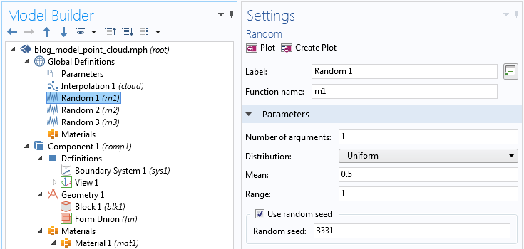
Start by generating three random variables with uniform distribution, with the Range set to 1 and the Mean value set to 0.5.
To generate this type of plot, we use a Scatter Volume plot type. This is available by right-clicking a 3D Plot Group and selecting More Plots > Scatter Volume.
In the Settings window of the Scatter Volume plot, set the expression for the X-, Y-, and Z-components: rn1(x), rn2(x), and rn3(x), respectively. Here, we are using the x-coordinate in an unusual way, in that we are using it merely as a long vector of arbitrary values.
Next, in the Evaluation Points section, set the Number of points for the X grid points to 100,000; 1,000,000; or more, depending on how many points your computer can handle. Set each of the Y grid point and Z grid point values to 1. This is a trick for getting a long vector of values that we can feed into the random functions in order to generate a lot of random points within the unit cube.

To make the plot appear as in the above figure, go to the Radius section and set Expression to cloud(rn1(x),rn2(x),rn3(x)) and the Radius scale factor to 0.3. In addition, in the Color section, set the Expression to cloud(rn1(x),rn2(x),rn3(x)) and the Color table to GrayScale.
One additional noteworthy fact about this plot: negative values will be ignored. This helps our visualization, since roughly half of the generated data is negative and we can more easily see through the data and get an intuitive feel for the variations. This method will only work for a rectangular block. To instead generate this type of plot over an arbitrary CAD geometry, you can use the Particle Tracing Module, which allows you to generate random points inside any type of CAD model.
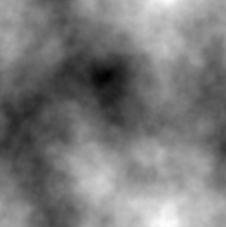
By the way, a similar-looking plot can be achieved in a 2D model by simply creating a 2D Surface plot using a double-sum expression, as shown in the figure above.


Comments (20)
Rehema Ndeda
June 24, 2017Thank you for the post. It has been quite useful.
Yu Zhang
April 2, 2018Hi, Bjorn:
Thank you for sharing us this method to generated random field. Now I am going to generate a Gaussian field (mean 0, and variance 1) which is spatial correlated, and found that the fast Fourier Transformation is commonly used to generate such a random field. I am not sure whether I can use your method to create a spatial correlated Gaussian field which has mean 0 and variance 1. In you method, is the generated f(x,y) just the Gaussian field I wanted to create?
Thank you for your time and help.
Yu
Bjorn Sjodin
April 3, 2018Hi Yu,
Thanks for your comment. The method described here is more or less equivalent to an FFT-based method. However, this method will of course not scale as well as an FFT-based method. You will find a comparison between the two methods in a previous blog posting:
https://www.comsol.com/blogs/how-to-generate-random-surfaces-in-comsol-multiphysics/
in the section called
Relationship to Discrete Cosine and Fourier Transforms
There you will also find a book reference for the FFT-based method.
Some benefits with the method used in this blog post are: a) ease-of-use b) mesh independence, you can refine the mesh and get consistent results without redefining the random process.
Best regards,
Bjorn
Yu Zhang
April 4, 2018Hi, Bjorn:
Thank you so much for your detailed reply, which helped me get more insights about the this method. However, I am still have some confusions about it. Could you please give me a further explanation? Any help would be highly appreciated.
(1) How does the autocorrelation function (like Gaussian type rho(h)=exp(-(h/b)^2), where b is the correlation length) relate to the parameters (like k, l, m) in your method?
(2) After the transform, does the generated random field still have standard Gaussian distribution (mean 0, and variance 1)?
Thank you so much for your time and help.
Yu
Bjorn Sjodin
April 4, 2018Hi Yu,
1)
The relationship between the continuous variables x, y, and z and the discrete k,l, and m are:
x=k/(2K+1)
y=l/(2L+1)
z=m/(2M+1)
To compare with the usual way of writing discrete transforms you may need to look at the previous blog post again
https://www.comsol.com/blogs/how-to-generate-random-surfaces-in-comsol-multiphysics/
where we also describe the index shift that you can perform in the discrete Fourier transform.
When all that is sorted out you need to make sure you have a fine enough mesh to resolve the individual cos (or sin) functions for the highest frequencies.
We need to remember here that we are performing these calculations on an unstructured triangulated/tetrahedrized mesh instead of a structured grid as in the discrete case.
With finite elements (such as in COMSOL) those cos functions are approximated with a piecewise polynomial on each element. By refining the mesh you should in theory get as good autocorrelation as your computer can handle a fine mesh. The finer the mesh the closer to the “exact” autocorrelation you will get.
2) The mean will be 0 but the variance calculation will not be 1. For example, the arbitrary factor 0.01 in front of the series is controlling the variance and the more terms you include the greater the variance. I haven’t looked for a literature reference for what the variance is in terms of this type of truncated Fourier series, or tried to derive it, but it would certainly be interesting to see such an expression. Perhaps some reader would know the answer to this question before any of us have looked it up. If I can find a nice expression for this I will make sure to post it here.
Bjorn
Bjorn Sjodin
May 8, 2020 COMSOL EmployeeThere is an update and answer to the question 2 above about how to get the variance from this type of function.
The files that are available for download as part of the blog post https://www.comsol.com/blogs/how-to-generate-random-surfaces-in-comsol-multiphysics/ now contains a file random_flat_surface_roughness.mph (made with version 5.5) . This is a geometry part file and you can, for example, copy it to the part library at:
C:\Program Files\COMSOL\COMSOL55\Multiphysics\parts\COMSOL_Multiphysics\Random_Surfaces
This part will allow you to specify the surface roughness by an amplitude scaling factor (the “old” way) or the surface RMS height (Sq). The method used to give the surface RMS height demonstrates how to control the standard deviation or, more or less equivalently, variance of this type of data and is also applicable to this posting on 3D random data. You just need a triple sum instead of a double sum. The file shows how to scale the amplitude to get a function that is proportional to the standard deviation.
Bjorn
Bjorn Sjodin
April 4, 2018Hi again Yu,
I think for understanding the correlation for Fourier synthesis methods, like this one, case you can read
The Science of Fractal Images, Editors: Peitgen, Heinz-Otto, Saupe, Dietmar. Eds.
which is the book referenced in the first blog posting. Describing this here would be too much to fit in this comment field and more of text book chapter character.
Then you also have the discretization error described in the above comment coming from the finite element method, so only when the mesh element size goes to zero you would get perfect agreement with the “exact” theory of text books.
Bjorn
Yu Zhang
April 4, 2018Hi, Bjorn,
Thanks a lot for your generous help and detailed explanations. I will study the book systematically. If I have some new findings, I will post it here. Thank you.
Best regards,
Yu
Tuan Tu NGUYEN
March 23, 2020Hi Bjorn,
Thank you for the post ! It’s was very useful ! However, I’m wondering if the method is still valid for the case when I already have a distribution of the properties ? (it means actually it’s no longer be something randomly distributed in the spatial domain). In this case, how could we randomly distribute the properties (with knowing distribution) over a surface or volume ?
Could we replace the gaussian distribution g1 by a distribution of the parameter we want to use ?
Best
Tu
Bjorn Sjodin
March 23, 2020 COMSOL EmployeeHi Tu,
I’m glad you liked the post. Do you mean that you have a known distribution function for your random properties? In that case, do you have a mathematical description of this distribution?
Bjorn
Tuan Tu NGUYEN
March 23, 2020Thank Bjorn for your quick reply.
Indeed, as you said, I know the distribution of my properties (as a look-up table, but I can try to fit with an explicit function if needed).
To be more specific, for ex when I used the li-ion battery physics, I’d like to load the particle size distribution instead of a mean radius, and so the same for the conductivity, the diffusivity, etc…
Bjorn Sjodin
March 24, 2020 COMSOL EmployeeHi Tu,
Without knowing the details of your application, I think you can use techniques similar to those in this blog post to approximate distribution functions based on Normal (or Gaussian) distribution functions. In this posting an approximate probability distribution is generated by a sum of Normal distribution functions. In a similar way you can approximate a wide range of probability distributions based on COMSOL’s built-in random function. I suggest you search the web for references on such techniques.
Bjorn
Tuan Tu NGUYEN
March 24, 2020Thank you for the suggestion. I’ve found this thread https://www.comsol.com/blogs/sampling-random-numbers-from-probability-distribution-functions/#eq2 , that can actually solve my problem.
For the coefficient 0.01, it’s arbitrary taken I suppose ? And if I don’t want to have a negative values In my results, what should I change in this case ?
Thank you,
Best,
Tu
Bjorn Sjodin
March 27, 2020 COMSOL EmployeeHi Tu,
For this specific problem and for further discussions I suggest you contact our technical support team.
Best regards,
Bjorn
Eduardo Moreno
June 19, 2020Do you have and mph example for the case of Randomized Inhomogeneous Material Data for 2D axial symmetric?
best regards
Eduardo Moreno
Bjorn Sjodin
June 22, 2020 COMSOL EmployeeHi Eduardo,
We don’t have any examples of axial symmetry yet. Could you tell me a bit more about your application? This may be something we could cover by a future blog post.
Best regards,
Bjorn Sjodin
Diletta Giuntini
August 11, 2020Hello Bjorn,
Thank you for this post, very useful.
I implemented this approach to generate an initial condition that is randomly distributed in space (3D). However, when I then use the cloud function into my problem’s geometry (an elongated bar), the random distribution does not occupy my entire domain, but only a small portion – even if I scale the expression as you suggested in the wrench expression above. Any insight, or should I perhaps share my model with the technical support?
Bjorn Sjodin
August 11, 2020 COMSOL EmployeeHi Diletta,
I’m glad you found it useful. Probably some translation of the random data is also needed in your case. Usually you can accomplish this by replacing expressions in x, y, and z with corresponding expressions in x-x0, y-y0, and z-z0 where x0, y0, z0 is some kind of representative center of the geometry. In addition, you may need scaling and even potentially rotation on top of that. If you need further help don’t hesitate contacting technical support.
Best regards,
Bjorn
Rukshan Azoor
August 25, 2020Hi Bjorn,
This and your previous article have been very useful. I just wanted to share another method that I eventually adopted to generate spatially correlated random field realisations to be input into COMSOL (feel free to remove this comment if not relevant).
I used a Python library to generate a spatially correlated Gaussian random field with mean 0 and variance 1 (similar to what Yu required above), so I can transform it to the required material property. I have described the method and shared the code here:
https://rukshanmaliq.blogspot.com/2020/06/modelling-soil-inhomogeneity-using-3d.html
The code can be used in a Jupyter notebook and the spatial correlation lengths, size of domain and the resolution can be changed. The output is a point cloud text-file that can be imported directly into COMSOL as an interpolation function as you have done.
Also, is there an easy method that you could suggest to automate the process of importing data, running and saving results for multiple realisations?
Thanks!
Rukshan
Bjorn Sjodin
August 26, 2020 COMSOL EmployeeHi Rukshan,
I’m glad you liked the articles. Automating this is possible by using the COMSOL API for use with Java, for example using the Method Editor in the Application Builder, or with MATLAB, using the LiveLink for MATLAB product.
I hope this helps,
Bjorn