

We often need to work with experimental data in COMSOL Multiphysics, usually to represent material properties or other inputs to our model. However, experimental data is often noisy; it contains experimental errors that we do not want to introduce into our simulations. In this blog post, we will look at how to fit smooth curves and surfaces to experimental data using the core functionality of COMSOL Multiphysics.
Curve Fitting as a Minimization Problem
Let’s take a look at some sample experimental data in the plot below. Observe that the data is noisy and that the sampling is nonuniform in the x-axis. This experimental data may represent a material property. If the material property is dependent upon the solution variable (such as a temperature-dependent thermal conductivity), then we would usually not want to use this data directly in our analyses. Such noisy input data can often cause solver convergence difficulties, for the reasons discussed here. If we instead approximate the data with a smooth curve, then model convergence can often be improved and we will also have a simple function to represent the material property.
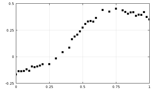
Experimental data that we would like to approximate with a simpler function.
What we would like to do is find a function, F(x), that fits the experimental data, D(x), as closely as possible. We will define the “best-fit” function as the function that minimizes the square of the difference between the experimental data and our fitting function, integrated over the entire data range. That is, our objective is to minimize:
So the first thing that we need to do is to make some decisions about what type of function we would like to fit. We have a great deal of flexibility about what type of functions to use, but we should choose a fitting function that results in a problem which will be numerically well-conditioned. Although we will not go into the details about why, for maximum robustness we will choose to fit this function:
which in this case, for a=0, b=1, simplifies to:
Now we need to find the four coefficients that will minimize:
Although this may sound like an optimization problem, we do not have any constraints on our coefficients and we will assume that the above function has a single minimum. This minimum will correspond to the point where the derivatives, with respect to the coefficients, are zero. That is, to find the best fit function, we must find the values of the coefficients at which:
It turns out that we can solve this problem with the core capabilities of COMSOL Multiphysics. Let’s find out how…
The COMSOL Implementation
We start by creating a new file containing a 1D component. We will use the Global ODEs and DAEs physics interface to solve for our coefficients and we will use the Stationary Solver. For simplicity, we will use a dimensionless length unit, as shown in the screenshot below.
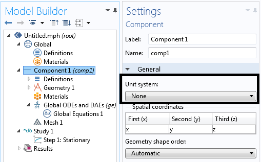
Start out with a 1D component and set Unit system to None.
Next, create the geometry. Our geometry should contain our interval (in this case, the range of our sample points is from 0 to 1) as well as a set of points along the x-direction for every sample point. You can simply copy and paste this range of points from a spreadsheet into the Point feature, as shown.
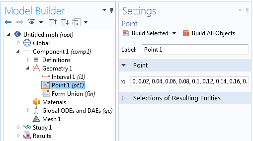
Add points over the interval at every data sample point.
Read in the experimental data using the Interpolation function. Give your data a reasonable name (we simply use D in the screenshot below), check on the “Use spatial coordinates as arguments”, and make sure to use the default Linear interpolation between data points.
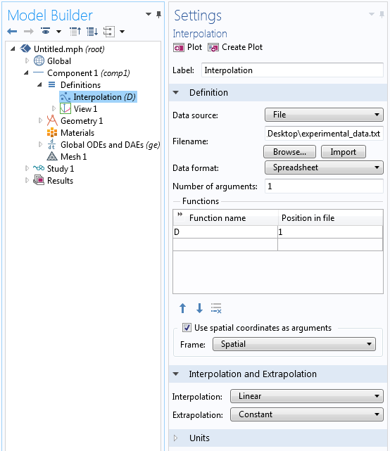
The settings for importing the experimental data.
Define an Integration Operator over all domains. You can use the default name: intop1. This feature will be used to take the integral described above.
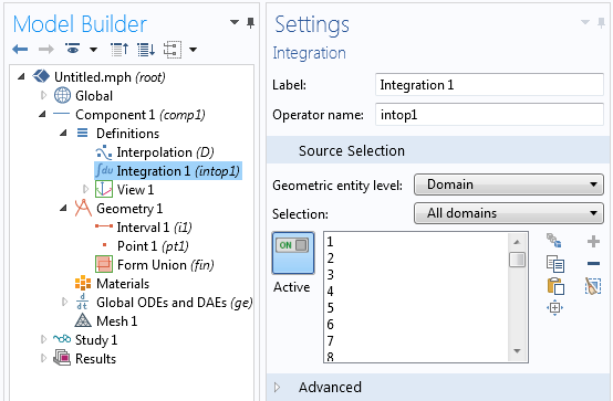
The Integration Operator is defined over all domains.
Now define two variables. One will be your function, F, and the other will be the function that we want to minimize, R. Since the Geometric Entity Level is set to Entire Model, F will be defined everywhere and spatially varying as a function of x. On the other hand, R is scalar valued everywhere and also available throughout the entire model. As shown in the screenshot below, we can enter F as a function of c_0,c_1,c_2,c_3 and will define these coefficients later.
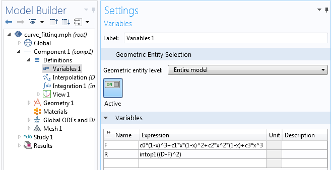
The definition of our fitting function and the quantity we wish to minimize.
Next, we can use the Global Equations interface to define the four equations that we want to satisfy for our four coefficients. Recall that we want the derivative of R with respect to each coefficient to be zero. Using the differentiation operator, d(f(x),x), we can enter this as shown below:
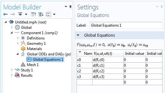
The Global Equations that are used to solve for the coefficients of our fitting function.
Finally, we need to have an appropriate mesh on our 1D domain. Recall that earlier we placed a geometric point at each data sampling point. Using the Distribution subfeature on the Edge Mesh feature, we can ensure that there is one element between each data point. We do not need any more elements than this, since we are assuming linear interpolation between data points, but we do not want less than this, because then we will miss some of the experimental data points.

There should be one element over each data interval.
We can now solve this stationary problem for the numerical values of our coefficients and plot the results. From the plot below, we can see the data points with the linear interpolation between them, as well as the computed fitting function. We have minimized the square of the difference between these two curves, integrated over the interval, and now have a smooth and simple function that approximates our data quite well.
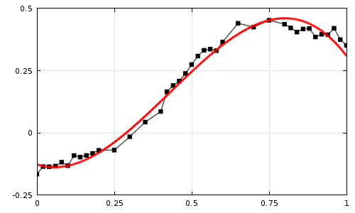
The experimental data (black, with linear interpolation) and the fitted function (red).
Further Extensions
Now, what we’ve done so far is actually fairly straightforward and you could compute similar types of curve fits in a spreadsheet program or any number of other software tools. But there is much more that we can do with this approach. We are not limited to using this fitting function. You are free to choose any function you want, but it is best to use a function that is a sum of set of orthogonal functions. Try out, for example:
Be aware, however, that you will only want to solve for the linear coefficients on the various terms within the fitting function. You would not want to use nonlinear fitting coefficients such as F(x) = c_0 + c_1sin ( \pi x /c_3 ) + c_2cos ( \pi x /c_4 ) since such a problem might be too highly nonlinear to converge.
And what if you have a 2D or 3D data set? You can actually apply the exact same approach as we’ve outlined here. The only difference is that you will need to set up a 2D or a 3D domain. The domains need not be Cartesian and you can even switch to a different coordinate system.
Let’s take a quick look at some sample data points measured over the region shown below:
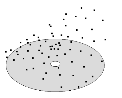
Sampled data in a 2D region. We want a best fit surface to the heights of these points.
Since the data is sampled over this annular region and seems to have variations with respect to the radial and circumferential directions (r,\theta), rather than the Cartesian directions, we can try to fit the function:
We can follow the exact same procedure as before. The only difference being that we need to integrate over a 2D domain rather than a line and write our expression using a cylindrical coordinate system.
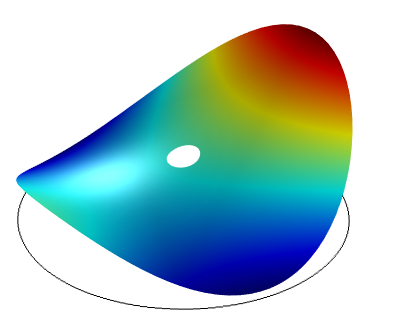
The computed best-fit surface to the data shown above.
Closing Remarks
You can see that the core COMSOL Multiphysics package has very flexible capabilities for finding a best-fit curve to data in 1D, 2D, or 3D using the methods shown here.
There can be cases where you might want to go beyond a simple curve-fit and want to consider some additional constraints. In that case, you would want to use the capabilities of the Optimization Module, which can also perform these types of curve fits and much, much more. For an introduction to the Optimization Module for curve fitting and the related topic of parameter estimation, please also see:


Comments (1)
Zhidong Zhang
May 16, 2019Hi Walter,
If I have the measured and the computed curves in the same plot, how can I calculate R^2 in Comsol?
Thanks.
Best regards,
Zhidong