
Rotating components are important elements in machines such as gas turbines, turbochargers, pumps, compressors, electric generators, and motors. Designing such a component requires studying its critical speed, which is the speed at which the amplitude of the vibration in the system becomes large — often leading to failure. Let’s explore how to find the critical speeds for a wide range of rotors via the Rotor Bearing System Simulator, created using the COMSOL Multiphysics® software.
What Is the Critical Speed of a Rotor?
A critical speed is the angular speed of a rotor that matches one of its natural frequencies. Finding the natural frequencies of a stationary rotor, however, is not enough to determine the critical speed. The real challenge comes from the fact that the natural frequency of the rotor depends on the rotor angular speed. Therefore, it is important to compute the natural frequency of a rotating component by considering the effect of the rotation.
This effect can be automatically included in the underlying model of a COMSOL app, which shows only the important design parameters as inputs. Let’s see how we can find the critical speeds of various rotating systems using an example from the Application Gallery: the Rotor Bearing System Simulator.
Video demonstrating the Rotor Bearing System Simulator.
Exploring the Rotor Bearing System Simulator App
A typical rotor system has three standard components:
- Rotor, also called the shaft
- Disks
- Bearings
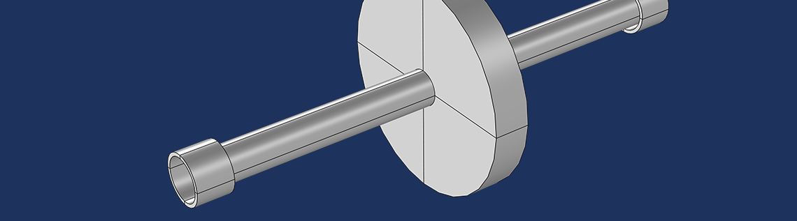
A rotor system, which includes a rotor (shaft), disk, and bearing.
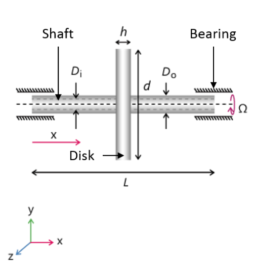
In most cases, the shaft is either a solid or hollow cylinder on which various components are mounted. In rotordynamics terminology, these mounted components are often called disks and they are modeled as rigid objects due to their high stiffness when compared with the shaft. Therefore, only inertial properties of the disks are important in the critical speed analysis. Shafts are flexible elements and also have inertia. A complete specification of the shaft requires its geometric dimensions and material properties, such as Young’s modulus, Poisson’s ratio, and density. Bearings are the components on which the shaft is supported. These components are described by their equivalent stiffness and damping coefficients.
Now, let’s see how this information is passed to the app. There are various sections in the app for different uses, including:
- Inputting data
- Evaluating results
- Accessing information
The sections to specify the input data are Rotor Properties, Disks, Bearings, and Study Parameters. The Critical Speeds section is used to evaluate the critical speed of the modeled rotor. The Geometry State and Information sections contain the information about the geometry and the solver, respectively. On the right panel of the app, the geometry of the rotor, whirl plot, and Campbell plot can be accessed. Various items on the top ribbon are provided to perform the different actions in the app.

The user interface of the Rotor Bearing System Simulator.
In the Rotor Properties section, you can specify the geometric dimensions of the rotor (shaft) and its material properties. There are two ways to specify the material properties of the rotor:
- Choose the material of the rotor from the combo box that has a list of standard materials. In this case, material properties are automatically assigned to the rotor, corresponding with the selected material.
- Choose the user-defined option in the combo box mentioned above and then specify the material properties of the rotor.
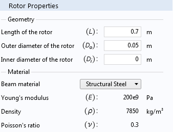
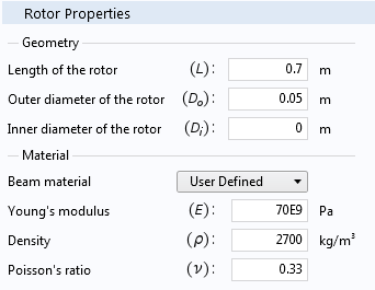
The Rotor Properties section, with a material from the list (left) and a user-defined material (right).
The Disks section has a combo box to either specify the geometric dimensions of the disks together with the density or to specify the inertial properties directly. The properties of disks can be given as tabular data in which each row in the table represents the disk. You can add as many rows as there are disks on the rotor. If Geometric dimension is chosen, then the location of the disk, outer diameter, thickness, and density can be specified. For Inertial properties, you can specify the location, mass, polar, and diametral moment of inertia.
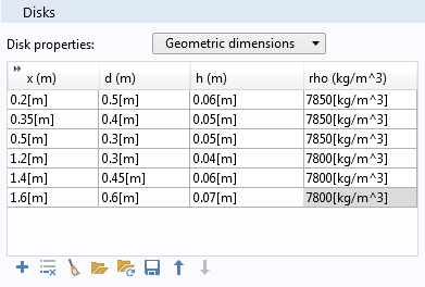
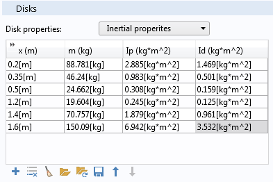
The Disks section, showing the properties specified through geometric dimensions (left) and mass and moment of inertia (right).
Data entered in the table can be saved to a file for later use. Also, if you have a text file of the disk data in the appropriate format, it can be directly imported into the Disks table, thus simplifying the process of entering data.
You can specify the bearings’ stiffness and damping coefficients in the Bearings section. This section again requires a tabular input, with each row representing a bearing. Cross-coupled stiffness (kyz and kzy) and damping coefficients (cyz and czy) for the bearing can also be specified (if available). These coefficients play an important role in determining the stability of the bearing. Tabular input for the bearing, like the disk, has the advantage of saving the data for later use and also importing the data from a text file.
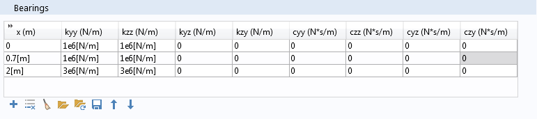
The Bearings section.
After you are done setting up the system properties, you can evaluate the rotor system to be analyzed by updating the geometry.
The Study Parameters section provides you with the inputs to specify the maximum angular speed of the rotor and the steps in the parametric sweep of the angular speed from zero to the maximum value. You can also specify the number of natural frequencies to be computed by the app.
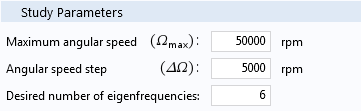
The Study Parameters section is used to specify the angular speed and eigenfrequency information.
Computing Critical Speeds
As discussed above, the critical speed of a rotor is determined by obtaining the variation of the natural frequency with its angular speed. To do so, after setting up the model, you first perform an eigenfrequency analysis by clicking the Compute button. As a result, in the Graphics window, you can see the whirl, orbit, and Campbell plots for the modeled rotor system. In the Campbell plot, critical speeds are the points where the frequency is equal to the angular speed. In other words, critical speeds are the intersection points of the eigenfrequency curves with the ω = Ω curve, as shown below.
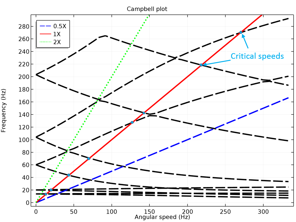
In the Campbell plot, critical speeds are marked as points (light blue).
In the underlying model, there is no direct way of calculating the critical speed. This is where you harness the power of the Application Builder. Using the Method Editor (available in the Application Builder), you can easily write your own method to compute the critical speeds. This is what is done in the Rotor Bearing System Simulator. A screenshot of the code for computing the critical speed is shown in the figure below.
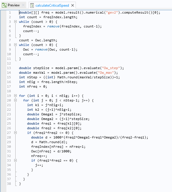
The code shows how the critical speed is calculated.
The calculated critical speeds are then displayed as a table in the Critical Speeds section.
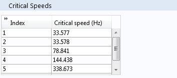
The Critical Speeds section.
Bringing Apps into the Design Process
Simple apps such as this can help designers to quickly come up with a good starting point for their design. Further, the app allows them to test various configurations without spending excessive money on experiments. Apps also make such investigations convenient because they hide the technical details while highlighting the important parameters in the design process. This provides designers with the accessibility and flexibility to control the design parameters and evaluate their findings with only a few clicks and without worrying about the underlying technical details.
Apps are not limited to modeling only simple physics. The underlying model for an app could be as complex as possible, simulating multiple physics simultaneously. The app itself could further extend the model, with the help of the Method Editor, to bring the simulation closer to reality.
Further Resources
- Learn about using the Rotordynamics Module:
- Watch this archived webinar to find out how to use the Rotordynamics Module


Comments (7)
Anonymous
June 7, 2017Can you give detail how to make the APPs by PDF or video? Thank you very much!
Bridget Cunningham
June 9, 2017Hello,
Thank you for your comment.
We do have a variety of resources available on how to build apps. To get started, you can consult this introductory manual: http://www.comsol.com/documentation/IntroductionToApplicationBuilder.pdf. You can also check out this video series on the blog: https://www.comsol.com/blogs/tag/intro-to-application-builder-videos/.
If you have any additional questions on building apps, please contact our Support team.
Online Support Center: https://www.comsol.com/support
Email: support@comsol.com
Van-The Than
July 1, 2017If I have not created the APP. How can I set the stiffness of bearing for rotor dynamics simulation? Could you guide me find the option in this module? Thank you very much!
Van-The Than
July 1, 2017Dear Sir,
If I have not created the APP, how can I set the value of stiffness during simulated rotor dynamic? Could you please guide me to key in the stiffness in this module? Thank you very much!
Prashant Srivastava
July 6, 2017Dear Van-The,
If you want to set the stiffness in a rotordynamics model, you need to add ‘Journal Bearing’ feature in either of the ‘Solid Rotor’ and ‘Beam Rotor’ interfaces. By default you will have ‘No clearance’ bearing model but to specify the stiffness you need to change the bearing model to ‘Total spring and damping constant’. Once you do that you can specify translational and rotational bearing stiffness and damping constants.
I hope this answers your question. To know more about it you can write to us at support@comsol.com. You can also go through Rotordynamics Module’s user guide from page 52-63 and 106-110 on bearing modeling.
Shuai Zhu
July 25, 2017Hi,
A group of MCGILL gives the steps of matrix extract by ANSYS, see http://structdynviblab.mcgill.ca/pdf/AnsysMatlab.pdf
Does Comsol export the matrix, as well ?
If so, can you give me some comments?
Future questions, the matrix are used for some time-marching method, the results can be imported into COMSOL for figure ?
Thanks
Best, Hamilton
Prashant Srivastava
July 26, 2017Hi Shuai,
Short answer to your question is, yes you can extract the mass, damping and stiffness matrices and many other matrices in COMSOL. For the detailed answer, we suggest that you forward your question to support@comsol.com.
Thanks,
Prashant