Heat Transfer Module

Analyze Thermal Effects with Advanced Simulation Software

Analyze heat transfer by conduction, convection, and radiation with the Heat Transfer Module, an add-on product to the COMSOL Multiphysics® simulation platform. The Heat Transfer Module includes a comprehensive set of features for investigating thermal designs and effects of heat loads. You can model the temperature fields and heat fluxes throughout components, enclosures, and buildings. To examine the real-world behavior of a system or design virtually, easily couple multiple physical effects in one simulation with the multiphysics modeling capabilities included in the software.

Contact COMSOL
A model image of an LED bulb showing the fluid flow around the bulb and the temperature and fluid flow inside the bulb.

Modes of Heat Transfer

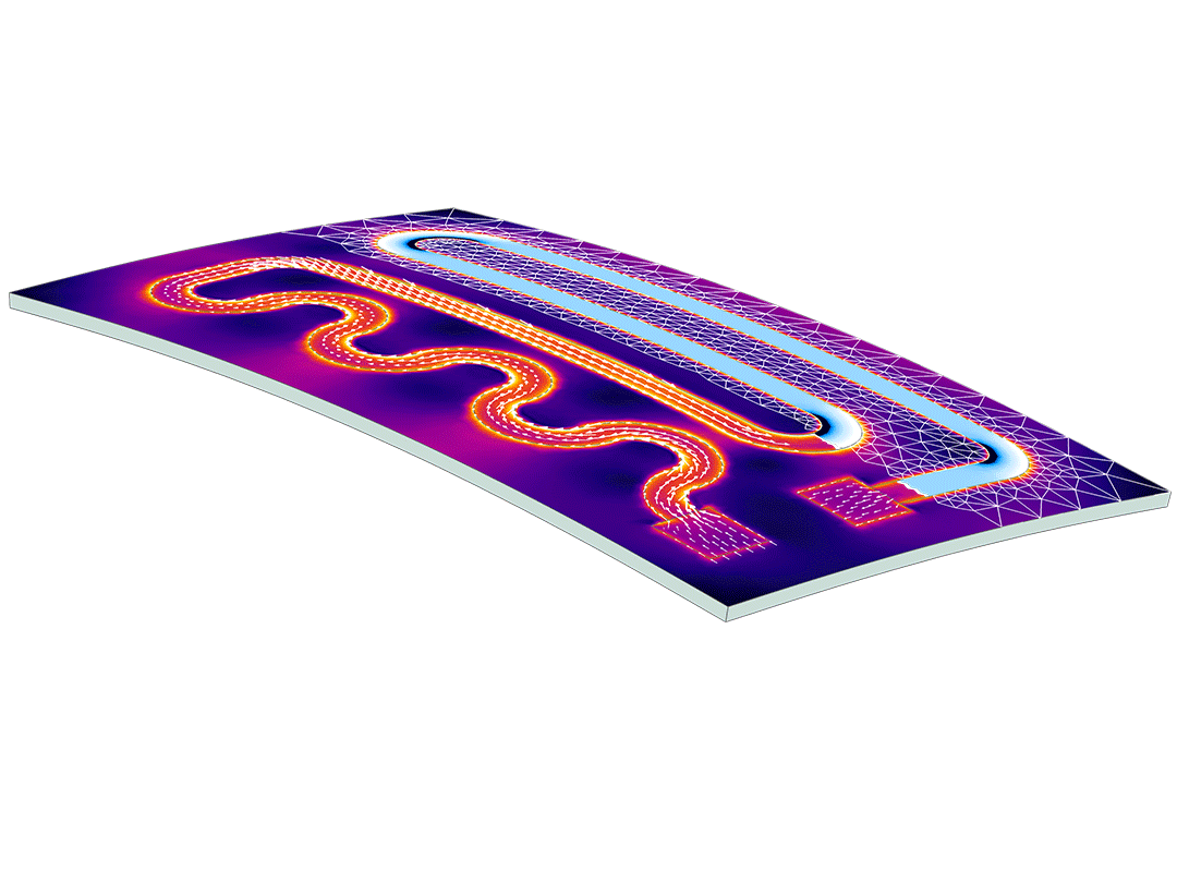
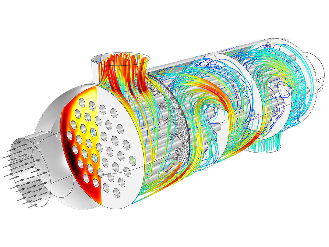
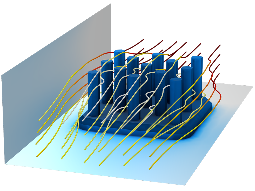
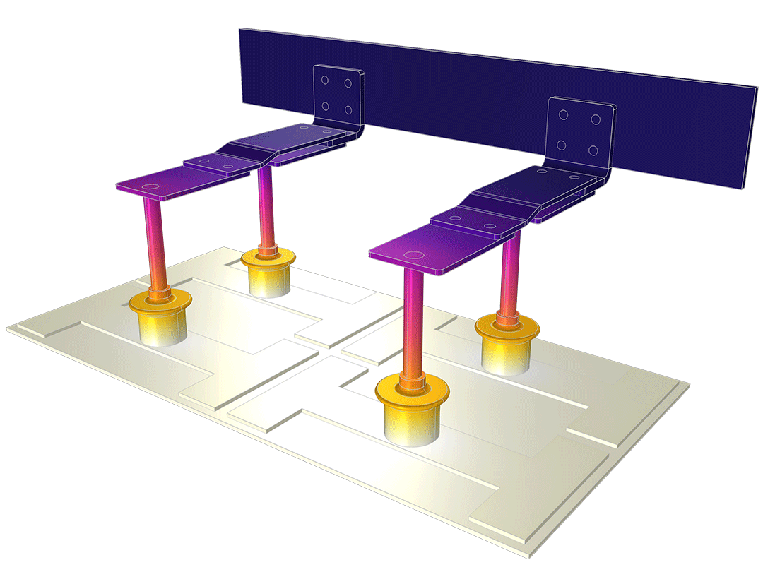
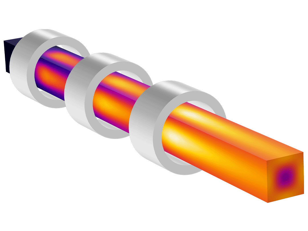
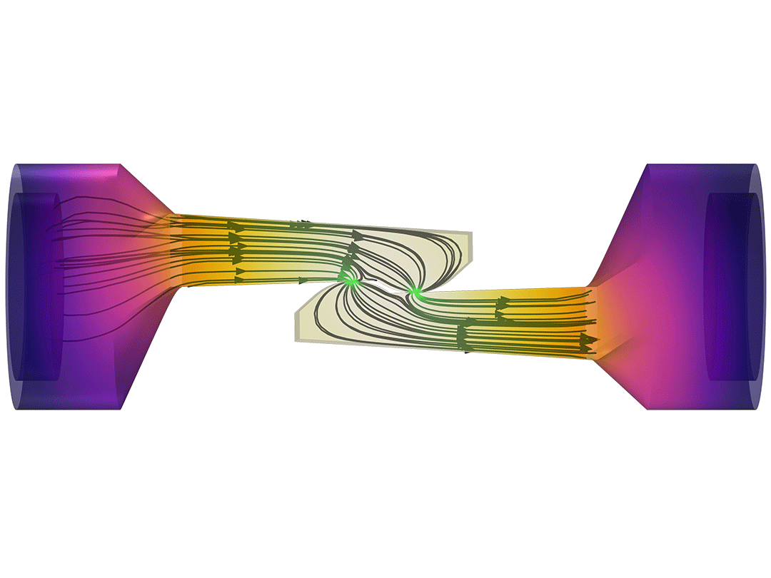
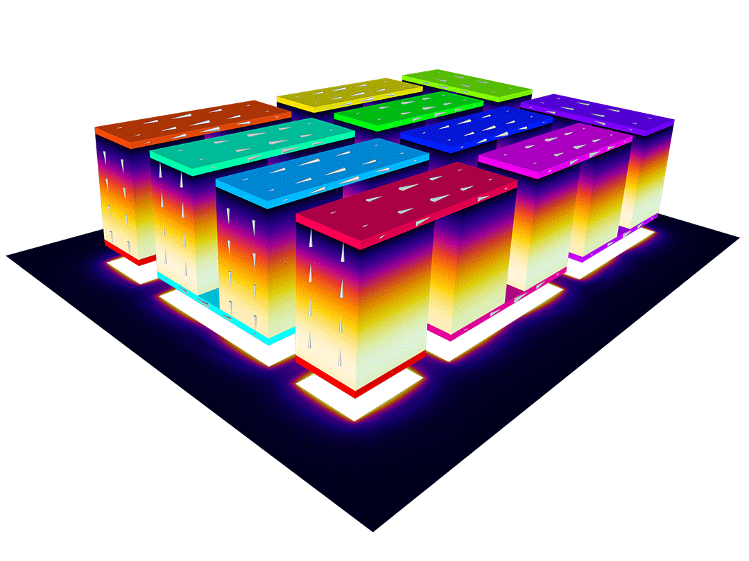
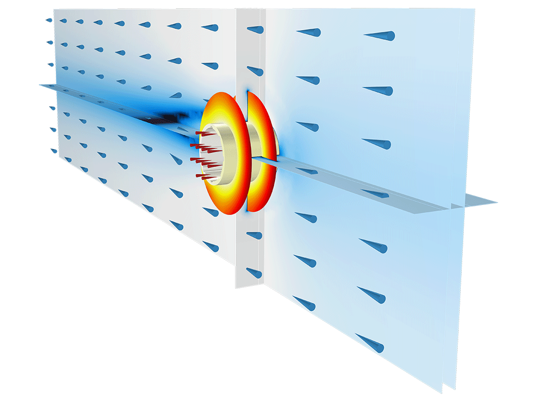
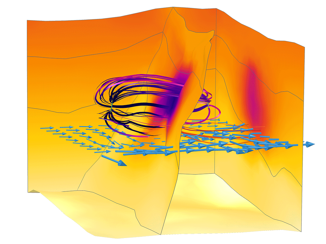
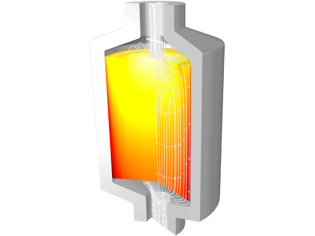
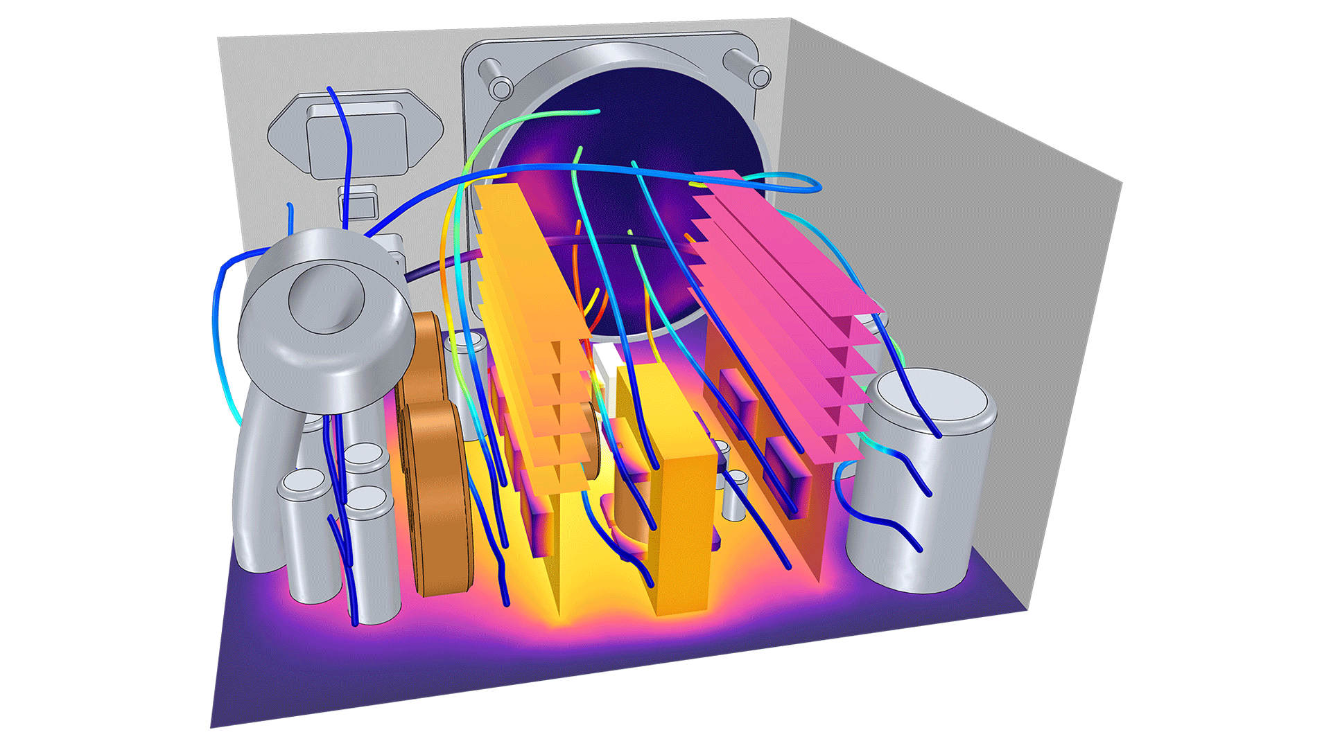
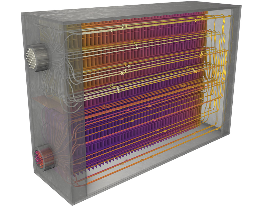
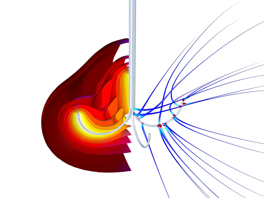
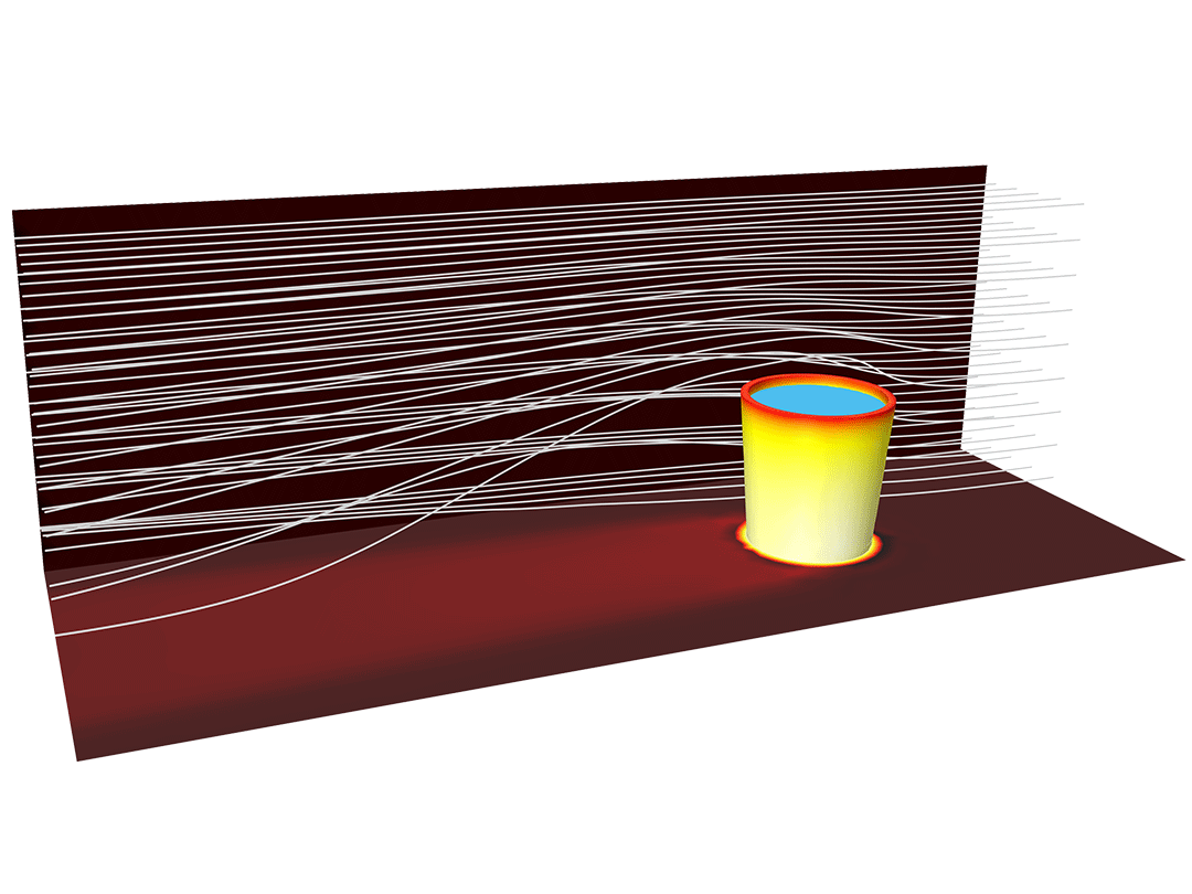
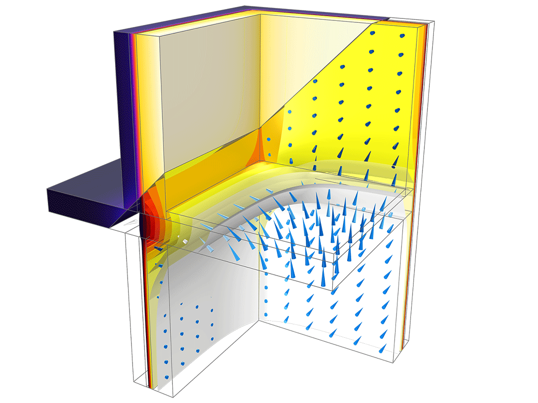
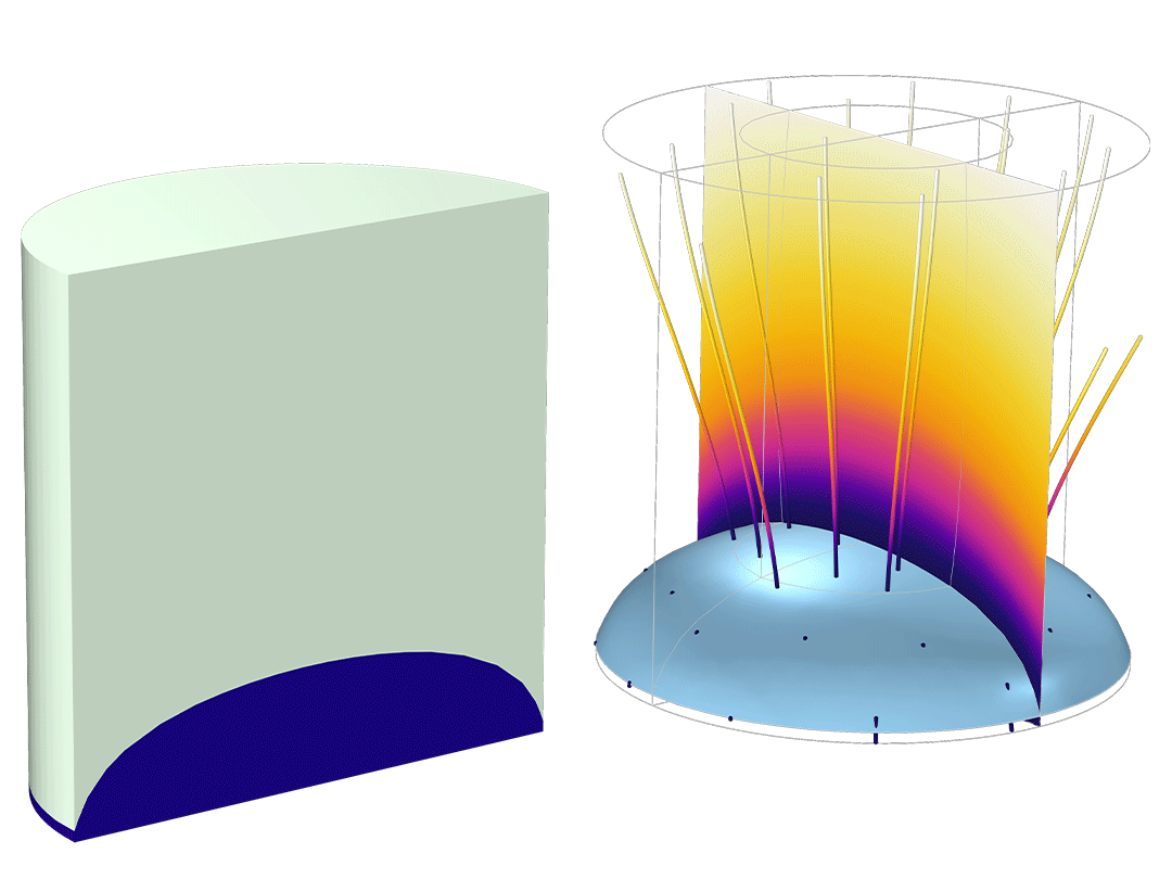
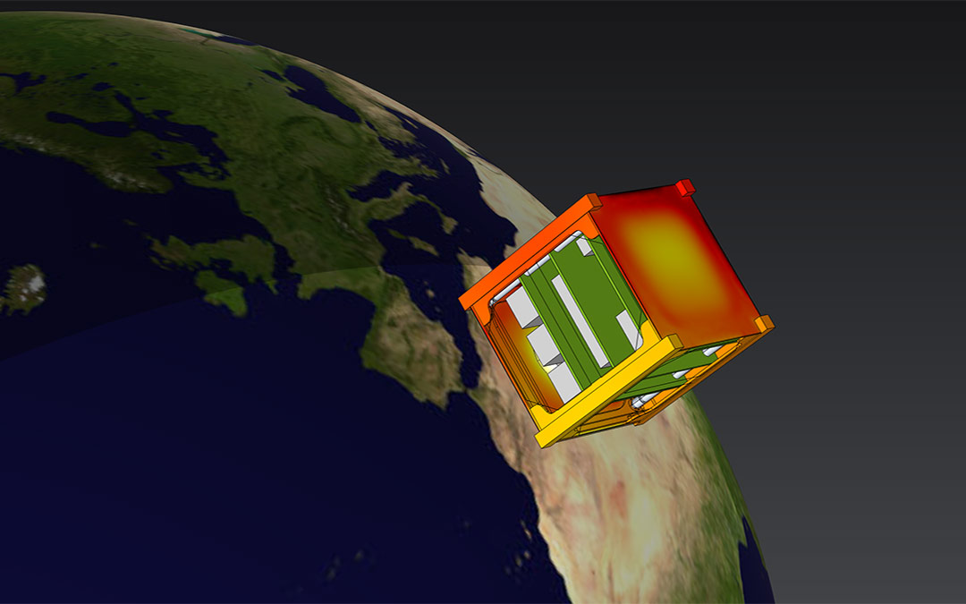
All of the capabilities in the Heat Transfer Module are based on the three modes of heat transfer: conduction, convection, and radiation. Conduction in any material can have an isotropic or anisotropic thermal conductivity, and it may be constant or a function of temperature. Convection, the motion of fluids in heat transfer simulations, can be forced or free (natural) convection. Thermal radiation can be accounted for using surface-to-surface radiation or radiation in semitransparent media.

There are many variations within the modes of heat transfer, and the different modes must be considered together — in some cases, all three at once. All of this requires different equations that must be handled simultaneously to ensure accurate models. The Heat Transfer Module is developed to handle any type of heat transfer you are looking to model.

What You Can Model with the Heat Transfer Module

A multiphysics modeling approach for the many types of heat sources you may be interested in simulating.

A detailed view of a busbar assembly showing the temperature distribution.

Joule Heating

Model Joule heating (also known as resistive heating) in solids, fluids, shells, and layered shells.

A detailed view of the temperature distribution in a steel billet as it passes through three energized coils.

Induction Heating1

Model inline induction heaters and metal processing applications.

A model of a waveguide bend that is partially transparent to reveal a red-white-and-blue surface plot representing the wave traveling through and a dielectric block with temperature shown in red, yellow, and white color gradient.

Microwave Heating2

Model microwave, or RF, heating in waveguides, tissue, and other bio-applications.

A detailed view of half a glass cylinder showing the beam intensity in one quarter and the temperature distribution in the other quarter.

Laser Heating3

Use the Beer–Lambert Law to model laser heating and ablation in various manufacturing and biomedical processes.

A detailed view of a turbine stator blade showing the temperature distribution.

Thermal Stress4

Understand the effects of thermal expansion and thermal stress for a variety of operating conditions.

A detailed view of the electric current streamlines through a contact switch and the temperature distribution.

Thermal Contact

Include the contact thermal conductance coefficient, which depends on the contact pressure from the solid mechanics model.

A detailed view of a thermoelectric cooler device showing the temperature distribution.

Thermoelectric Effects

Account for the Peltier–Seebeck–Thomson effects, and include common materials, such as bismuth telluride and lead telluride.

A detailed view of a finned-pipe heat exchanger showing the flow past the pipe and the temperature in the fins.

Thin Shells

Analyze thermal performance when designing electronic devices and power system components.

A detailed view of the flow and heat transfer through a fracture in a geothermal doublet.

Heat Transfer in Porous Media

Account for conduction and convection in a porous media, as well as thermal dispersion.

A detailed view of a storage tank showing the flow and heat transfer through the tank.

Local Thermal Nonequilibrium

Simulate heat transfer in porous media where a local thermal equilibrium is not assumed, as with a rapid flow in the pores.

A detailed view of a computer's power supply unit with a fan and grille showing the fluid flow through the unit and heat transfer in the components.

Electronic Cooling

Analyze cooling capacity with efficient and accurate simulations, to avoid malfunction and suboptimal designs.

A close-up view of a plate-fin heat exchanger model in the Heat Camera Light color table.

Heat Exchangers

Analyze fluids carrying energy over large distances, while the solids separate the fluids to exchange energy without mixing.

A detailed view of an electric probe with electric current streamlines and temperature isosurfaces of the surrounding tissue.

Medical Technology and Bioheating

Use the bioheat equation to analyze processes in medical applications: tumor ablation, skin probes, and tissue necrosis.

A detailed view of a glass of hot water showing the temperature of the glass cup and the streamlines through a flow channel passing by the cup.

Evaporative Cooling

Model heat and moisture transport in air to determine saturation pressure, account for evaporation, and avoid condensation.

A model of a building structure part with the temperature distribution throughout shown in the Heat Camera color table and heat flux shown as arrows.

Thermal Management in Buildings

Analyze thermal performance of wooden frames, window frames, porous building materials, and other building structures.

A detailed view of two cylinders are shown to demonstrate the freeze drying process: the two phases in one cylinder and the heat transfer in the other.

Freeze Drying

Compute coupled heat and mass balances to simulate an advancing fluid–solid interface through a porous medium.

A close-up view of a satellite on an Earth model.

Spacecraft Thermal Analysis

Compute the spacecraft temperature from the direct solar radiation, albedo, and planet infrared flux as well as the radiative heat transfer between various spacecraft parts.

  1. Requires the AC/DC Module
  2. Requires the RF Module
  3. Requires the Wave Optics Module
  4. Requires the Structural Mechanics Module or MEMS Module

Features and Functionality in the Heat Transfer Module

The Heat Transfer Module offers specialized functionality for modeling heat transfer effects and works seamlessly in the COMSOL Multiphysics® platform for a consistent model-building workflow.

The settings window for the Nonisothermal Flow multiphysics coupling and the results of the heat sink simulation.

Conjugate Heat Transfer and Nonisothermal Flow

The Heat Transfer Module contains features for modeling conjugate heat transfer and nonisothermal flow effects. Laminar and turbulent flow are both supported and can be modeled with natural and forced convection. To account for natural convection, simply select the Gravity check box. Pressure work and viscous dissipation can also be activated to affect the temperature distribution.

Turbulence can be modeled using Reynolds-averaged Navier–Stokes (RANS) models such as the k-ε, low-Reynolds k-ε, algebraic yPlus, or LVEL turbulence models. The realizable k-ε, k-ω, shear stress transport (SST), v2-f, and Spalart–Allmaras turbulence models are available when combined with the CFD Module. The temperature transition at the fluid–solid interface is automatically handled using continuity, wall functions, or automatic wall treatment, depending on the flow model.

The Phase Change Interface feature settings and the Graphics window showing application of the Phase Change Interface.

Phase Change

To simulate phase change phenomena in heat transfer analyses, the Heat Transfer Module provides two methods. The Phase Change Material feature implements the apparent heat capacity formulation and accounts for enthalpy of phase change and changes in material properties. This method includes the ability to model volume and/or topology changes.

Alternatively, the Phase Change Interface feature models phase change following the Stefan energy balance condition to compute the velocity of the interface between two phases that may have different densities. Combined with deformed geometry, this approach is very efficient and effective when there is no topology change.

The Layered Thermal Expansion multiphysics interface and the temperature and deformation results in the Graphics window.

Thin Layers and Shells

For heat transfer in thin layers, the Heat Transfer Module provides individual layer models and layered material technology, to investigate heat transfer in layers that are geometrically much smaller than the rest of a model. This functionality is available for thin layers, shells, thin films, and fractures.

For individual layers, the thermally thin layer model is used for highly conductive materials with heat transfer tangential to the layer and negligible temperature difference on either side of the layer. Conversely, the thermally thick layer model can represent poorly conducting materials that act as a thermal resistance in the shell's perpendicular direction; this model computes the temperature difference between the two layer sides. Finally, the general model provides a highly accurate and universal model, as it embeds the complete heat equations.

The layered material technology includes preprocessing tools for detailed layered material definition, load/save of layered structure configurations from/to a file, and layer preview features. You can visualize the results in thin, layered structures as if they were originally modeled as 3D solids. The layered material functionality is included in the AC/DC Module and the Structural Mechanics Module, making it possible to include multiphysics couplings like electromagnetic heating or thermal expansion on layered materials. Moreover, the Thermal Connection multiphysics couplings can be used to define a continuity condition between two temperature fields, computed by a domain heat transfer interface and a Heat Transfer in Shells interface, respectively.

The Model Builder showing the Lumped Thermal System interface and Lumped System Connector feature highlighted, as well as the results comparison graph.

Lumped Thermal Systems

Features are available for computing the heat transfer rate and temperature distributions in a thermal network. The Lumped Thermal System interface supports lumped features such as thermal resistors, heat rate, and thermal mass. The software solves an energy conservation equation using the temperatures and heat rates as dependent variables.

The Surface-to-Surface Radiation interface in the Model Builder and the Graphics window showing the simulation results: surface radiosity of a parasol and coolers in the sun.

Surface-to-Surface Radiation

The Heat Transfer Module provides features for modeling surface-to-surface radiation on diffuse surfaces, mixed diffuse-specular surfaces, and semitransparent layers. These features are available for 2D, 2D axisymmetric, and 3D geometries. Between the surfaces, in the cavities, the exposure to radiation can be evaluated using the Fluence Rate feature.

Predefined settings are available for solar and ambient radiation, where the surface absorptivity for short wavelengths (the solar spectral band) may differ from the surface emissivity for the longer wavelengths (the ambient spectral band). In addition, the sun radiation direction can be defined from the geographical position and time.

The view factors are computed using the hemicube, the ray-shooting, or direct integration area method. For computationally effective simulations, it is possible to define planes or sectors of symmetry. When combined with a moving frame, the surface-to-surface radiation interface automatically updates the view factors as the geometrical configuration deforms.

The Radiation in Participating Media interface settings and the Graphics window showing the incident radiation in a glass plate.

Radiation in Semitransparent Media

With the Heat Transfer Module, you have the tools to simulate many types of radiation in semitransparent media: participating media, absorbing and scattering media, and beams in absorbing media.

For radiation in participating media, use the Rosseland approximation, P1 approximation, or discrete ordinate method (DOM). For radiation in absorbing and scattering media, use the P1 approximation and DOM to, for example, model light diffusion in a nonemitting medium. Lastly, you can model a radiative beam in absorbing media using the Beer–Lambert law, and couple the effect with other forms of heat transfer.

The three moisture transport multiphysics couplings and the results of the evaporative cooling of a glass of water showing the vapor concentration.

Moisture Transport

Heat and moisture transport requires extensive multiphysics capabilities to couple heat transfer with moisture flow, moisture transport in building materials, moist air, and hygroscopic porous media. To study these effects, the Heat Transfer Module includes settings for modeling moisture transport in air and moist porous media coupled with nonisothermal flow. There are tools to analyze water condensation and evaporation on surfaces, and additional features to analyze heat and moisture storage, latent heat effects, as well as diffusion and transport of moisture.

A close-up view of the Planet Properties settings and a satellite model in the Graphics window.

Orbital Thermal Loads

For radiative loads and temperature on a spacecraft, the Orbital Thermal Loads interface provides ready-made features for modeling the radiation from the Sun and Earth for satellites orbiting around Earth. This feature makes it possible to include the spacecraft radiative properties, orbit and orientation, orbital maneuvers, and planet properties. In addition, the interface computes and generates results that show direct solar radiation, albedo, and planet infrared flux as well as the radiative heat transfer between the different spacecraft parts. The interface can be combined with a heat transfer interface to account for heat conduction in a spacecraft's solid parts.

Every business and every simulation need is different.

In order to fully evaluate whether or not the COMSOL Multiphysics® software will meet your requirements, you need to contact us. By talking to one of our sales representatives, you will get personalized recommendations and fully documented examples to help you get the most out of your evaluation and guide you to choose the best license option to suit your needs.

Just click on the "Contact COMSOL" button, fill in your contact details and any specific comments or questions, and submit. You will receive a response from a sales representative within one business day.

Next Step

Request a Software Demonstration