
Wrinkling is a subject of research that spans from space engineering, where it pertains to inflatable antennas, to bioengineering, where it pertains to the familiar wrinkling of skin. Regardless of the field they work in, engineers and researchers who deal with thin structures are familiar with the underlying mechanism of wrinkling: a lack of stiffness or reduced stiffness when a thin structure is subjected to compressive stresses. In this blog post, we will explore how to model wrinkling using the COMSOL Multiphysics® software.
Introduction
In structural simulations, thin structures are typically modeled using either shell or membrane elements. Shell elements take into account the bending stiffness of the structure, while membrane elements do not. This fundamental difference defines how these two types of elements handle the modeling of wrinkling. When bending stiffness is taken into account, as with shell modeling, wrinkling is observed at a critical compressive stress characterized by the bending stiffness. On the other hand, if bending stiffness is not considered, as with membrane modeling, wrinkling is observed at the onset of compressive stresses.
In both cases, wrinkling is considered an instability and is also known as local buckling. When modeling wrinkling with shell elements, postbuckling analysis becomes necessary. It’s worth noting that the mesh discretization and any geometric imperfections can significantly impact the final results. Shell modeling provides the advantage of obtaining detailed information about wrinkling characteristics, such as wavelengths and amplitudes. However, in many modeling scenarios, the detailed characteristics of wrinkling are not particularly relevant; instead, the primary objective is to avoid wrinkling in the problem area. In such cases, modeling wrinkling with membrane elements can be advantageous because the approach is computationally inexpensive and offers better numerical stability.
Below, we will visit these two modeling approaches one by one. In the context of COMSOL Multiphysics®, shell and membrane elements are modeled using the Shell and Membrane interfaces, respectively.

Another familiar example of wrinkling: in a sail. Photo by Karla Car on Unsplash. The original work has been modified.
Modeling with the Membrane Interface
Thin structures modeled with the Membrane interface are in one of three possible states when deformed:
- Taut — when both in-plane principal stresses are positive
- Slack — when both in-plane principal stresses are negative
- Wrinkled — when one of the in-plane principal stresses is negative
In the ordinary membrane theory, a full strain-energy formulation is used, which accounts for compressive stresses in the wrinkled regions — in turn leading to unstable equilibrium solutions. To avoid the equilibrium instability produced by compressive stresses, the modified membrane theory (based on the tension field theory) was developed. The modified membrane theory returns a uniaxial stress state in the wrinkled region and zero stress state in the slack region, thus avoiding the equilibrium instability. The modified membrane theory can be branched into two main approaches: modifications of the deformation tensor and modification of the constitutive relation.
Modified Deformation Tensor Formulation
To understand the wrinkling kinematics, consider the following illustration:
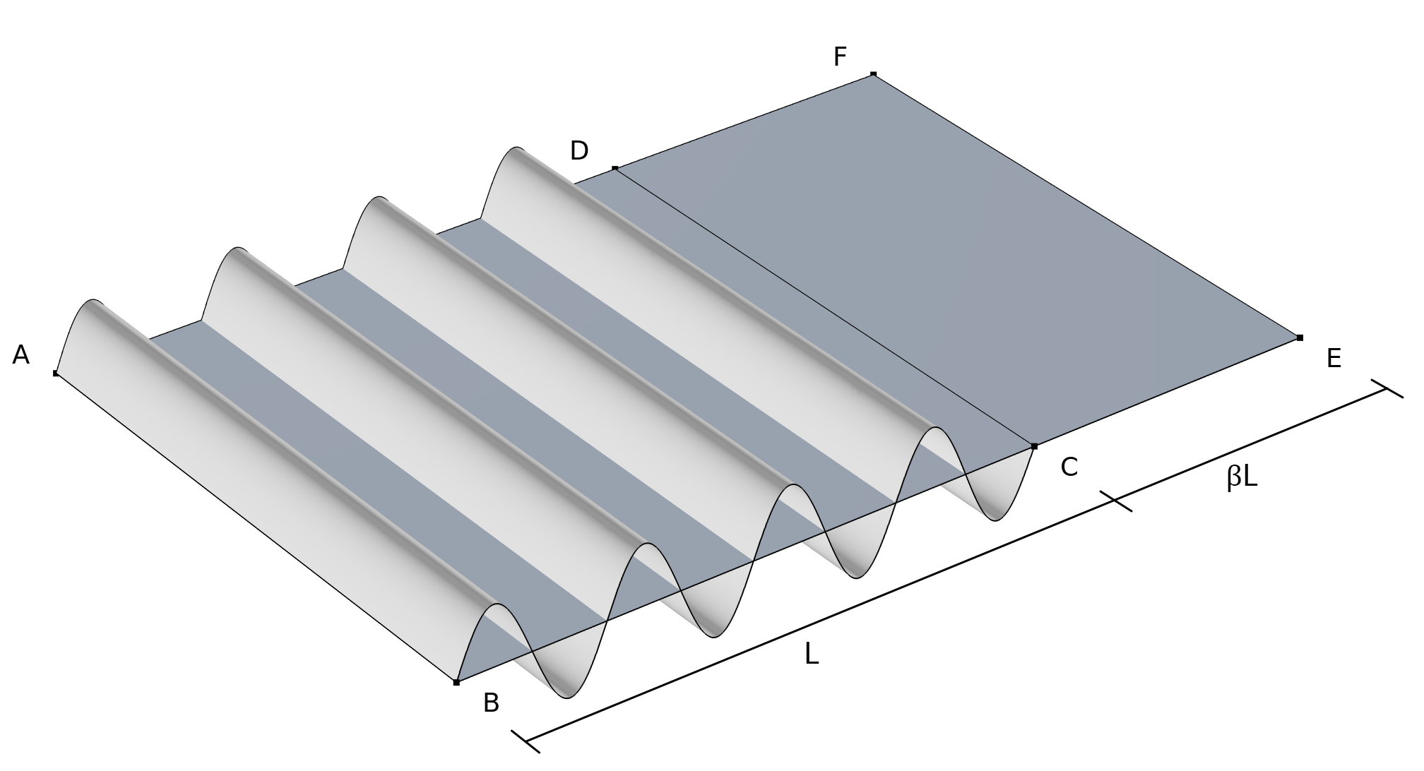
Kinematics of wrinkling. Curved surface ABCD represents the wrinkled configuration, planar surface ABCD represents the mean configuration, and planar surface ABEF represents the lengthened configuration.
For the wrinkled membrane, the figure above shows three different kinematic descriptions:
- The deformation tensor \widetilde{\bf{F}} maps the reference configuration to a true wrinkled configuration (curved surface ABCD).
- Not suitable for determining the strain field in the wrinkled membrane
- The deformation tensor \bf{F} maps the reference configuration to a mean configuration (planar surface ABCD), where the area is smaller than the actual wrinkled area.
- Not suitable for determining the strain field in the wrinkled membrane
- The deformation tensor \bar{\bf{F}} maps the reference configuration to a fictitious lengthened configuration (planar surface ABEF), where the area is equal to the actual wrinkled area.
- Suitable for determining the strain field in the wrinkled membrane
Assuming that wrinkling occurs in the \bf{n}_2 direction and that \bf{n}_1 is the direction of uniaxial tension, \bar{\bf{F}} is the modified deformation tensor and is written as
where \beta is a stretching/wrinkling parameter (Ref. 1). The \otimes symbol denotes the outer (dyadic) product of two vectors, producing a tensor. \beta=0 represents a taut condition. According to the orthogonality condition and tension field theory,
where \bf{\sigma} is the Cauchy stress. It is written in terms of the second Piola–Kirchhoff stress as
Assuming that the mean configuration is known (\bf{F}), the only unknowns are \bf{n}_2 and \beta.
Let’s map these equations into the reference configuration, which is more convenient, since the membrane kinematics and material properties are in the reference configuration. We will assume that \bf{h} is a vector in the reference configuration corresponding to the vector \bf{n}_2. Thus, the fictitious Green–Lagrange strain tensor \bar{\bf{E}} is written as
where \bf{C} is the mean right Cauchy tensor, \bf{N}_2 is the unit vector in the reference configuration, and \beta^* is the new wrinkling parameter.
The membrane surface is spanned by a coordinate system that has two in-plane orthogonal unit vectors, \bf{e}_1 and \bf{e}_2. \bf{N}_1 and \bf{N}_2 are written in terms of the angle \alpha as
The two nonlinear coupled equations to solve for two unknowns, \alpha and \beta^*, are
These two nonlinear algebraic equations can be solved using the Newton–Raphson method:
f_{1,\alpha} & f_{1,\beta^*}\\
f_{2,\alpha} & f_{2,\beta^*}
\end{pmatrix} \begin{pmatrix}
\Delta \alpha\\
\Delta \beta^*
\end{pmatrix} = \begin{pmatrix}
-f_1\\
-f_2
\end{pmatrix}.
Here, \alpha and \beta^* are solved by the local-level Newton–Raphson method at each Gauss point for each iteration at the global level.
The Wrinkling Feature
The modified deformation tensor approach is implemented in the built-in Wrinkling subnode, found under the Linear Elastic Material and Hyperelastic Material nodes in the Membrane interface. The Wrinkling subnode has three different options for a termination criterion of the local Newton–Raphson method, with the possibility to adjust the tolerances.
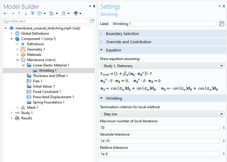
The Wrinkling subnode under the Linear Elastic Material feature.
There are several examples in the Application Gallery that show how to model wrinkling using the built-in functionality of the Membrane interface. A simple model that is easy to verify analytically is the Uniaxial Stretching of a Rectangular Membrane model. In this example, the numerical results are compared with the analytical results, as shown here:
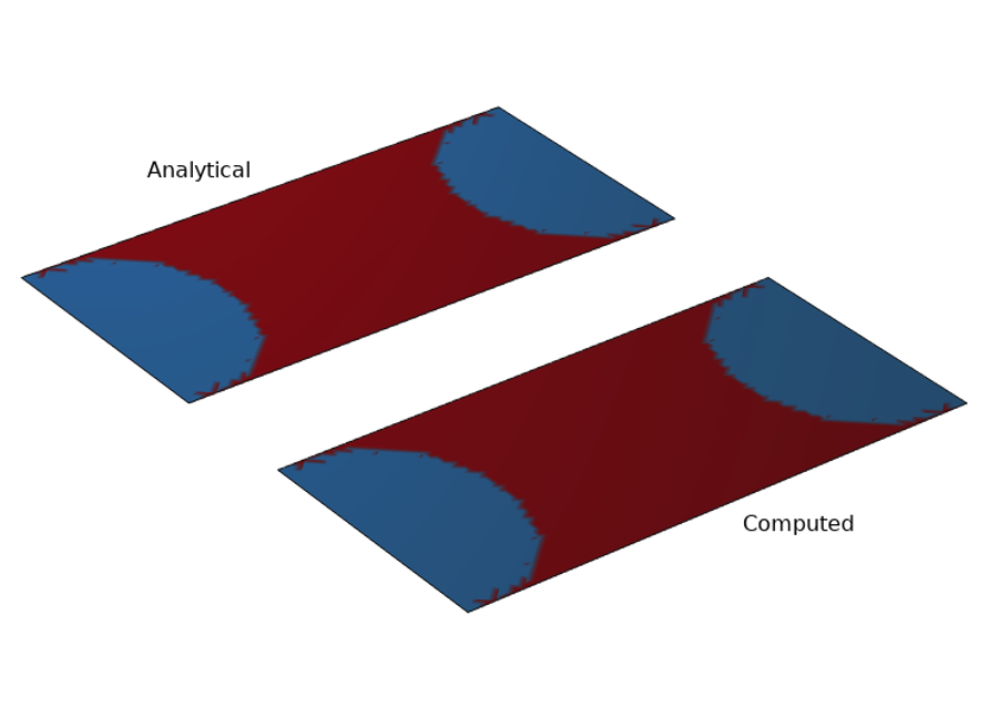
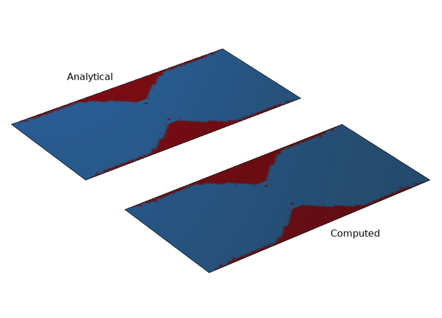
The wrinkled region of a rectangular membrane is shown in dark red. In the figure at left, an isotropic material is used, and in the figure at right, an orthotropic material is used. In both figures, the analytical results are compared with the computed (numerical) results.
The Inflation of a Square Airbag model is more practical and thus more complicated. The model demonstrates wrinkling in a square airbag during inflation with a linear elastic material. A similar model, Inflation of a Square Hyperelastic Airbag, uses a hyperelastic material.
Square airbag modeled with a linear elastic material. The wrinkled region is shown in dark red.
Another example that uses the built-in functionality of the Membrane interface to analyze wrinkling is the Torsion of a Circular Membrane model, in which a torque is applied to the inner edge only of an annulus to produce wrinkles. In this example, the impact of different mesh patterns and discretizations on the wrinkling patterns is observed.
Modified Constitutive Relation Formulation
As described above, the Wrinkling subnode in COMSOL Multiphysics® uses the modified deformation tensor formulation. However, thanks to the flexibility of the software, it is also possible to model wrinkling using the second approach: modifying the constitutive relation.
In this second formulation, the constitutive relation is modified for the wrinkled region. The strain energy used for the wrinkled region is called relaxed strain energy, while the strain energy used in the taut region is called full strain energy. This approach is applicable to all isotropic hyperelastic material models, but for simplicity a neo-Hookean incompressible material is considered here. The full strain energy density in terms of principal stretches \lambda_1 and \lambda_2 is written as
The principal Cauchy stress \sigma is given by
The principal Cauchy stress in each direction is given by
Let’s assume that the stretching occurs in the first principal direction and wrinkling occurs in the second principal direction. Then, the following equation must hold true in the wrinkled region:
This equation establishes a state of uniaxial stress in the wrinkled region, and the stress in the wrinkling direction becomes zero. Based on the zero stress in the wrinkling direction, the wrinkling condition in terms of principal stretches is obtained:
Hence, the wrinkling region is identified by the following inequality: \lambda_2 \sqrt{\lambda_1} < 1. Inserting the wrinkling condition obtained in terms of principal stretches in the full strain energy, the neo-Hookean relaxed strain energy is given by
The relaxed strain energy is not dependent on the stretch in the wrinkling direction; this means that the Cauchy stress in this direction will automatically become zero.
Using the wrinkling condition and the energy densities above, the strain energy density for the taut and wrinkled regions is written as
It can be shown that, for isotropic membranes, the modified deformation tensor and modified constitutive relation formulations are equivalent. (See Ref. 1 for more details.) However, the modified constitutive relation approach is applicable to isotropic membranes only, while the modified deformation tensor approach is more general and applicable to anisotropic membranes as well.
Comparing the Formulations in COMSOL Multiphysics®
In the Wrinkling of Cylindrical Membranes with Varying Thickness tutorial model, both formulations are compared and the results are found to be matching. In the model, the cylindrical membrane is first stretched axially and then inflated with water pressure. During the inflation, the outer edges are held fixed.
In COMSOL Multiphysics®, the modified constitutive relation formulation can be implemented by selecting the User Defined option of the Hyperelastic Material feature. Note that the strain energies of the neo-Hookean material in this tutorial model are written specifically for an incompressible isotropic membrane. In such a case, the built-in incompressibility formulation should not be used, since it adds extra terms that could cause a conflict. You can instead use the Compressible option in the user-defined hyperelastic material, which uses the given strain energy density exactly as written.
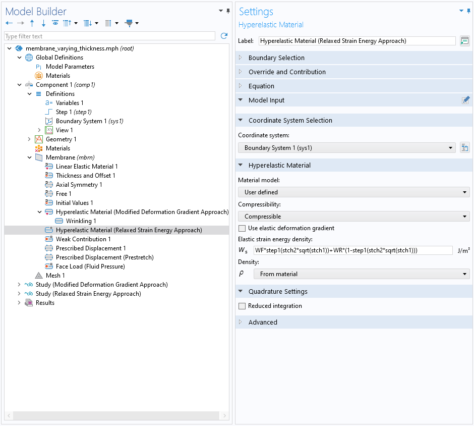
A Wrinkling subnode (which uses the modified deformation tensor formulation) and a user-defined hyperelastic material model (using the modified constitutive relation formulation).
The figures below show the wrinkled region of a cylindrical membrane at different water heights following both modeling approaches. The results presented show that both approaches are essentially equivalent and produce the same results.
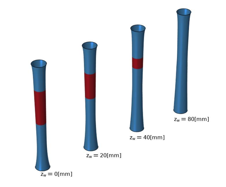
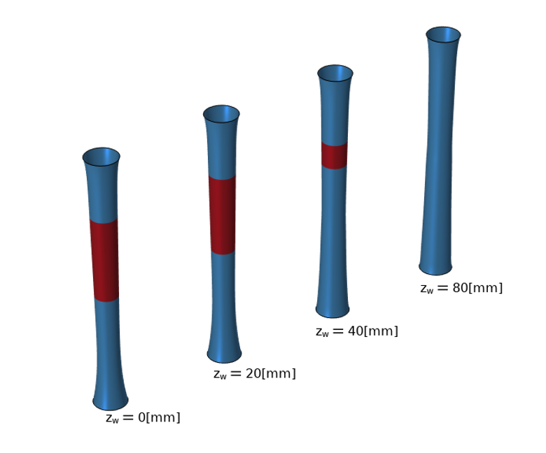
The wrinkled region of a cylindrical membrane is shown in dark red. At left, the modified deformation tensor approach has been used, and at right, the modified constitutive relation approach has been used. The annotation shows different fluid heights in the membrane, which is 80 mm tall with a 10-mm radius.
Modeling with the Shell Interface
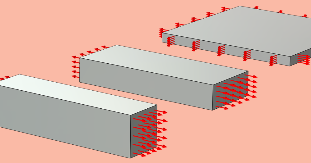
The treatment of wrinkling when using the Shell interface is based on bifurcation analysis. Wrinkling is considered a local buckling phenomenon due to the compressive stresses; hence, postbuckling analysis is required to model the wrinkling. The benefit of using postbuckling analysis is that the wavelengths and amplitudes of the wrinkling can be determined. The first step in the treatment of wrinkling is a prestressed eigenvalue analysis, where the potential buckling modes are identified. Then, the few selected buckling modes with proper scaling are used as a geometric imperfection for the postbuckling analysis.
In the Uniaxial Stretching of a Rectangular Sheet model, the occurrence of wrinkling in a thin rectangular sheet is studied using postbuckling analysis of shells. The following screenshot shows the model tree with the nodes needed for this analysis.

The Buckling Imperfection node and required studies for the Uniaxial Stretching of a Rectangular Sheet model.
The first step of this tutorial model involves identifying potential wrinkled regions using a static analysis. During this stage, the rectangular sheet is subjected to uniaxial stretching. The objective is to find the region where the second principal stress becomes compressive. Subsequently, a prestressed buckling analysis is performed using the Stationary and Linear Buckling study steps.
For postbuckling analysis, you can utilize the Buckling Imperfection node, as indicated in the screenshot above. Within this node, you have the option to select the desired number of buckling modes and their corresponding scaling factors. These scaled modes are then combined and applied as a geometric imperfection for the postbuckling analysis. From the Buckling Imperfection node, you can also create of a parametric nonlinear buckling study.
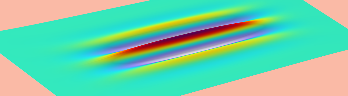
The animation below shows wrinkling in a rectangular sheet at increasing uniaxial strain, while the second figure shows the amplitude of the wrinkles along the central line in the wrinkling direction. Initially, when the strain is increased on the rectangular sheet, wrinkles start developing. The wrinkle amplitude increases with the increase in strain until it reaches a critical value, after which the wrinkle amplitude starts decreasing. At a certain strain value, the wrinkle amplitude becomes very small.
Wrinkles in a postbuckling analysis. The color scheme shows the wrinkle amplitude, where blue represents the negative range, red represents the positive range, and green represents zero displacement.
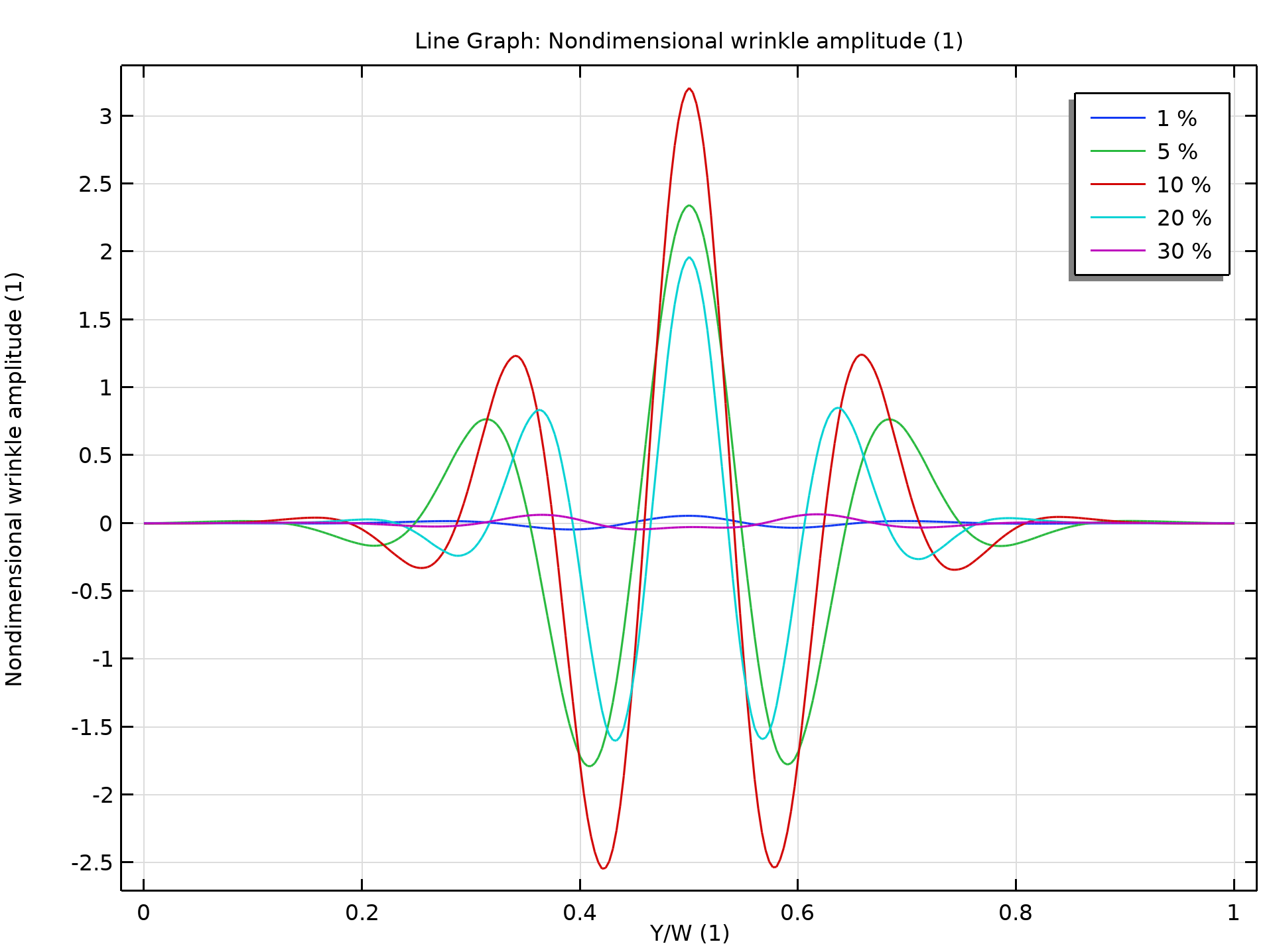
Wrinkle amplitude in a postbuckling analysis.
Concluding Remarks
As we’ve demonstrated, wrinkling can be modeled in COMSOL Multiphysics® using both the Membrane and Shell interfaces. Membrane analysis of wrinkling can be approached by modifying the deformation tensor or the constitutive relation. Membrane analysis is fast and numerically efficient, providing a correct identification of wrinkling regions and stress distribution. However, it does not provide information on wrinkle amplitudes and wavelengths. On the other hand, shell analysis of wrinkling is time-consuming, numerically demanding, and sensitive to geometric imperfection input. However, it provides valuable data on wrinkle amplitudes and wrinkle wavelengths, in addition to correctly predicting stress distribution and wrinkled regions. Because both types of analysis have their respective advantages and disadvantages, engineers can choose either type of analysis based on the specific modeling requirements.
References
- A. Patil, Inflation and Instabilities of Hyperelastic Membranes, PhD thesis, Royal Institute of Technology (KTH), Stockholm, 2016.
- H. Schoop et al., “Wrinkling of nonlinear membranes,” Computational Mechanics, vol. 29, pp. 68–74, 2002; https://doi.org/10.1007/s00466-002-0326-y

Comments (0)