

Microwave plasmas, or wave-heated discharges, find applications in many industrial areas such as semiconductor processing, surface treatment, and the abatement of hazardous gases. This blog post describes the theoretical basis of the Microwave Plasma interface available in the Plasma Module.
Introduction
Microwave plasmas are sustained when electrons can gain enough energy from an electromagnetic wave as it penetrates into the plasma. The physics of a microwave plasma is quite different depending on whether the TE mode (out-of-plane electric field) or the TM mode (in-plane electric field) is propagating. In both cases, it is not possible for the electromagnetic wave to penetrate into regions of the plasma where the electron density exceeds the critical electron density (around 7.6×10¹⁶ 1/m3 for 2.45 GHz). The critical electron density is given by the formula:
where \epsilon_0 is the permittivity of free space, m_e is the electron mass, \omega is the angular frequency, and e is the electron charge. This corresponds to the point at which the angular frequency of the electromagnetic wave is equal to the plasma frequency. The pressure range for microwave plasmas is very broad. For electron cyclotron resonance (ECR) plasmas, the pressure can be on the order of around 1 Pa, while for non-ECR plasmas, the pressure typically ranges from 100 Pa up to atmospheric pressure. The power can range from a few watts to several kilowatts. Microwave plasmas are popular due to the cheap availability of microwave power.
Microwave Discharge Theory
In order to understand the nuances associated with modeling microwave plasmas, it is necessary to go over some of the theory as to how the discharge is sustained. The plasma characteristics on the microwave time scale are separated from the longer term plasma behavior, which is governed by the ambipolar fields.
Electromagnetic Fields
In the Plasma Module, the electromagnetic waves are computed in the frequency domain and all other variables in the time domain. In order to justify this approach, we start from Maxwell’s equations, which state that:
(2)
(3)
where \mathbf{\tilde{E}} is the electric field (V/m), \mathbf{\tilde{B}} is the magnetic flux density (T), \mathbf{\tilde{H}} is the magnetic field (A/m), \mathbf{\tilde{J}_p} is the plasma current density (A/m2), and \mathbf{\tilde{D}} is the electrical displacement (C/m2). The tilde is used to denote that the field is varying in time with frequency \omega/2 \pi. The plasma current density can be approximated by this expression:
(4)
where e is the unit charge (C), n_e is the electron density (1/m3), and \mathbf{\tilde{v}_e} is the mean electron velocity under the following two assumptions (Ref 1):
- Ion motion is neglected with respect to the electron motion on the microwave time scale.
- The electron density is assumed constant in space on the microwave time scale.
The mean electron velocity on the microwave time scale, \tilde{\mathbf{v}}_e, is obtained by assuming a Maxwellian distribution function and taking a first moment of the Boltzmann equation (Ref 2):
(5)
where m_e is the electron mass (kg) and \nu_m is the momentum transfer frequency between the electrons and background gas (1/s). As pointed out in Ref 1, the equations are linear, so we can take a Fourier transform of the equation system. Taking a Fourier transform of equation (5) gives:
(6)
where the tilde has been replaced by a bar to reflect the fact that we are now referring to the amplitude of the fields. Multiplying both sides by -e n_e and re-arranging gives:
(7)
or, in a simpler form:
(8)
where
(9)
Equations (1) and (2) can be re-arranged by taking the time derivative of (2) and substituting in (1)
(10)
where \mu is the permeability, \sigma is given in equation (8) above, and the plasma relative permittivity set to one. The equation could also be recast where the relative permittivity is complex-valued and the plasma conductivity is zero (Ref 3). The convention employed throughout the Plasma Module is that the plasma conductivity is given by equation (8) and the plasma relative permittivity is set to 1.
Solving the above equation with appropriate boundary conditions allows for the power transferred from the electromagnetic fields to the electrons to be calculated:
(11)
where \mathbf{\bar{J}} is the total current density (the plasma current plus the displacement current density) and * denotes the complex conjugate.
Ambipolar Fields
In addition to the equation above, a set of equations are solved in the time domain for the electron density n_e, electron energy density n_{\epsilon}, plasma potential V, and all ionic and neutral species. For the electron density:
(12)
where the electron flux, \mathbf{\Gamma}_e (1/(m2s)), is given by:
(13)
where \mu_e is the electron mobility (m2/(V-s)) and D_e is the electron diffusivity (m2/s). Notice that \mathbf{E} given above has no tilde associated with it. The electric field in this case is a static electric field that arises due to the separation of ions and electrons in the plasma. This is often known as the ambipolar field, and causes loss of electrons and ions to the reactor walls on time scales much longer than the microwave time scale (microseconds rather than sub-nanoseconds). The electron energy density, n_{\epsilon}, is computed using a similar equation:
(14)
where the third term on the left-hand side represents heating or cooling of electrons depending on whether their drift velocity is aligned with the ambipolar electric field. The heating of electrons due to the microwaves is given by the last term on the right-hand side and is defined in equation (10). The electron energy flux is given by:
(15)
The mean electron energy is computed using \bar{\epsilon} = n_{\epsilon}/n_e, \mu_{\epsilon} is the electron energy mobility (m2/(V-s)), D_{\epsilon} is the electron energy diffusivity (m2/s), and the term S_{\epsilon} represents energy loss due to elastic and inelastic collisions. This term is a highly nonlinear function of the mean electron energy and also a function of the electron density, background number density, and plasma chemistry. The complexities of this source term are not relevant to this discussion, but more details are given in the Plasma Module User’s Guide. For each ion and neutral species, a similar drift-diffusion equation is solved for the mass fraction of each species, w_k:
(16)
where the subscript k indicates the kth species. The mass flux vector, \mathbf{j}_k, represents mass transport due to migration from the ambipolar field and diffusion from concentration gradients (kg/m2s) and R_k is the reaction source or sink (kg/m3s). Again, further details are available in the Plasma Module User’s Guide and are not relevant to this discussion.
Finally, Poisson’s equation is solved in order to compute the ambipolar electric field generated by the separation of charges:
(17)
where \rho_v is the space charge density (C/m3) and \rho_v = e(n_i^+-n_e-n_i^-) where n_i^+ is the total number of positive ions and n_i^- is the total number of negative ions.
To summarize, the Microwave Plasma interface solves equations (10), (12), (14), (16), and (17) along with a suitable set of boundary conditions.
TE and TM Mode Propagation
In 2D or 2D axisymmetric models, the electromagnetic waves propagate in either the transverse electric (TE) mode or the transverse magnetic (TM) mode. In the TE mode, the electric field is only in the transverse direction and the magnetic field in the direction of propagation. Therefore, COMSOL solves only for the out-of-plane component of the high-frequency electric field. In the TM mode, the magnetic field is in the transverse direction and the electric field only in the direction of propagation, so COMSOL solves only for the in-plane components of the high-frequency electric field.
TE Mode
In the TE mode, electrons do not experience any change in the high-frequency electric field during the microwave time scale. This means that the phase coherence between the electrons and electromagnetic waves is only destroyed through collisions with the background gas. The loss of phase coherence between the electrons and high-frequency fields is what results in energy gain for the electrons. Therefore, the momentum collision frequency is simply given by:
where \nu_e is the collision frequency between the electrons and neutrals.
TM Mode
The TM mode causes in-plane motion of the electrons on the microwave time scale, so in regions where the high-frequency electric field is significant (the contour where the electron density is equal to the critical density), the time-averaged electric field experienced by the electrons may be nonzero. This destroys the phase coherence between the electrons and the fields, causing the electrons to gain energy. This is an example of a nonlocal kinetic effect, which is difficult to approximate with a fluid model. However, since this effect is similar to collisions with a background gas, the nonlocal effects can be approximated by adding an effective collision frequency to the momentum collision frequency:
where \nu_{\textrm{eff}} is the effective collision frequency to account for nonlocal effects. This is discussed in more detail in Ref 1, where an effective collision frequency of no more than \omega/20 is suggested.
ECR Reactors
When modeling ECR (electron cyclotron resonance) reactors, another layer of complication is added to the problem. The electron transport properties become tensors and functions of a static magnetic flux density, which can be created using permanent magnets. The plasma conductivity also becomes a full tensor, and a highly nonlinear function of the static magnetic flux density. In addition, it is necessary to consider all three components of the electromagnetic field. Comprehensive details on how to set up and solve a model of an ECR reactor can be found in the Dipolar Microwave Plasma Source model documentation.
Using the Microwave Plasma Interface in the Plasma Module
The Microwave Plasma interface can be used to model the three types of wave heated discharges listed above, but some care is required when setting up such models. In the Microwave Plasma settings window, there are three options under “Electric field components solved for”:
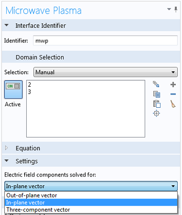
The options are as follows:
- Out-of-plane vector
- This corresponds to the TE mode
- In-plane vector
- This corresponds to the TM or TEM mode
- Three-component vector
- This is needed when modeling ECR reactors
Resonance Zone
The above equations are quite straightforward to solve, provided that the plasma frequency is below the angular frequency everywhere in the modeling domain. At a frequency of 2.45 GHz, this corresponds to an electron density of 7.6×10¹⁶ 1/m3, which is lower than most industrial applications. When the plasma density is equal to this value, the electromagnetic wave transitions from propagating waves to evanescent waves. Applications of microwave plasmas where the electron density is greater than the critical density include:
- Atmospheric pressure discharges, where the electron density can be several orders of magnitude higher than the critical density.
- Traveling-wave-sustained and surface-wave discharges. For the surface wave to propagate, the electron density must be higher than the critical density.
The resonance zone can be smoothed by activating the “Compute tensor plasma conductivity” checkbox in the Plasma Properties section:

The Doppler broadening parameter, \delta, corresponds to the value used for the effective collision frequency via the formula:
Therefore, a value of 20 is a compromise between accuracy and numerical stability as detailed above.
Deposited and Reflected Power
When using the Port boundary condition, the sum of the deposited and reflected power is supplied by default. In COMSOL Multiphysics version 4.4 it is also possible to specify only the deposited power, as shown in the settings window below:
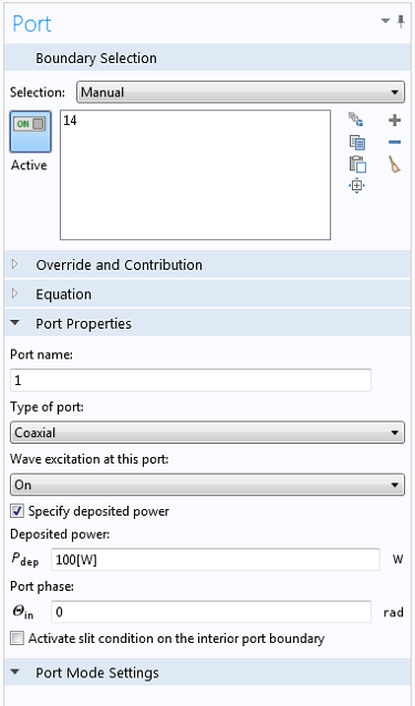
Using this option results in a more stable equation system because the total power transferred to the electrons remains constant. When the “Port input power” option is used, some of the power is deposited and some is reflected back out of the port, depending on the plasma’s current state. The plasma can go from absorbing a very small amount to a very large amount of power in a very short time period, which can make the problem numerically unstable or lead to the solver taking extremely small time steps.
Modeling Suggestions
The following is a collection of tips and tricks to try to help with convergence and decrease computation time:
- Fix the total power into the discharge by using the “Specify deposited power” option in the Port boundary condition, or by using the approach suggested in Ref 1 (demonstrated in the Dipolar Microwave Plasma Source model).
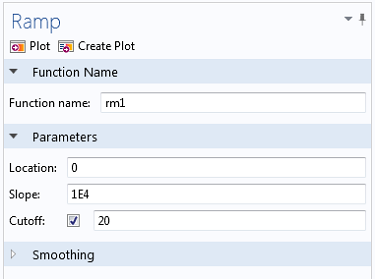
- Start the “Doppler broadening parameter” to a number below 1, then ramp this number up to 20 over the course of the simulation. This will smear out the resonance zone initially, then gradually make the region smaller and smaller. This can be implemented by defining a Ramp function with a cutoff value of 20.
- If the number density in the discharge is very high, it will probably be operating in full surface-wave mode. In this case, it may be necessary to use a doppler broadening parameter of 10. This will make the model more stable when solving, but the accuracy of such a model should be carefully considered.
- The initial electron density should be below the critical plasma density in the TM mode case. This recommendation is not strictly necessary for the TE mode case.
- Negatively biasing an electrode may have a significant effect on the discharge because it may shift the contour of critical plasma density away from its unbiased location. The best thing to do is to solve the model with a value of around 5 for the doppler broadening parameter, then slowly increase its value.
The following suggestions apply to all types of plasmas, but are worth mentioning again:
- The Debye length must be resolved adequately by the mesh. If your geometry is large (i.e. between 10 and 100 centimeters) and the electron density is very high (on the order of 1018 1/m3), then a very fine boundary layer mesh will be required close to the walls.
- Start with a simple plasma chemistry, like argon, before attempting a more exotic gas.
Solver Settings
Solver settings play an important role and COMSOL will automatically generate the best solver settings depending on how the model is set up. By default, when the “Port input power” option is used, the solver settings mentioned below are implemented. The segregated solver is used with two groups:
- All the plasma variables (electron density, electron energy, ion density, plasma potential, etc.)
- All the variables associated with the electromagnetic waves (high frequency electric field, S-parameters)
When the “Specify deposited power” option in the Port boundary condition is used, the solver suggestion is modified so that there are three groups:
- All the plasma variables (electron density, electron energy, ion density, plasma potential, etc.)
- All the variables associated with the electromagnetic waves (high-frequency electric field, S-parameters)
- A dependent variable called
Pdeposited, which is a differential algebraic equation used to fix the deposited, rather than total power
Example
An example of a TM mode microwave plasma can be found in the Model Gallery. The model uses an effective collision frequency of \omega/20, which smooths the region over which power is deposited to the electrons. As can be seen from the figure below, nearly all power deposition is still highly localized to the contour of critical electron density.
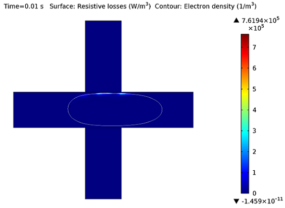
Plot of the power deposition into the plasma due to the high frequency fields. The white contour
is the contour of critical electron density.
Explore Further: Particle-Based Explanation of Collisionless Heating
Collisionless heating of electrons occurring in the TM mode can be demonstrated using the Particle Tracing Module. By starting an ensemble of particles with an initial mean energy of 0.5 eV on the contour of critical plasma density, the time evolution of the mean energy can be computed. The two plots below show how collisionless heating occurs in the TM mode, but not the TE mode.
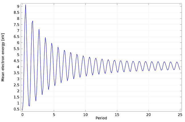
Plot of the mean electron energy for electrons in a TM mode collisionless plasma released on the contour of critical plasma density. There is a net energy gain even though there are no collisions.
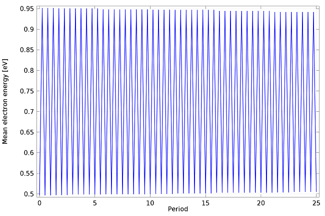
Plot of the mean electron energy for electrons in a TE mode collisionless plasma released on the contour of critical plasma density. There is no net energy gain over a number of RF cycles.
References
- G.J.M. Hagelaar, K. Makasheva, L. Garrigues, and J.-P. Boeuf, “Modelling of a dipolar microwave plasma sustained by electron cyclotron resonance,” J. Phys. D: Appl. Phys., vol. 42, p. 194019 (12pp), 2009.
- R.L. Kinder and M.J. Kushner, “Consequences of mode structure on plasma properties in electron cyclotron resonance sources,” J. Vac. Sci. Technol. A, vol. 17, Sep/Oct 1999.
- Michael A. Lieberman and Allan J. Lichtenberg, “Principles of Plasma Discharges and Materials Processing”, Wiley (2005).

Comments (1)
Enian Solomon
July 5, 2016Hello Daniel,
I have few questions on variables used in COMSOL’s Dipolar Microwave Plasma Source model. Under variables1> Psp (Total power absorbed by the plasma setpoint) and Pabs (Total power absorbed by the plasma).
1. What is this Psp (plasma setpoint) means?
2. If the desired Pabs=100W, then which value I need to use for Psp?
Thank you in advance!